Fast Fourier Transformation for polynomial multiplication

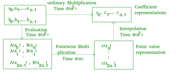
Given two polynomial A(x) and B(x), find the product C(x) = A(x)*B(x). There is already an O() naive approach to solve this problem. here. This approach uses the coefficient form of the polynomial to calculate the product.
A coefficient representation of a polynomial is a = a0, a1, ..., an-1.

Example-


Coefficient representation of A(x) = (9, -10, 7, 6)
Coefficient representation of B(x) = (-5, 4, 0, -2)

Input :
 A[] = {9, -10, 7, 6}
 B[] = {-5, 4, 0, -2}
Output : 

We can do better, if we represent the polynomial in another form.

Idea is to represent polynomial in point-value form and then compute the product. A point-value representation of a polynomial A(x) of degree-bound n is a set of n point-value pairs is{ (x0, y0), (x1, y1), ..., (xn-1, yn-1)} such that all of the xi are distinct and yi = A(xi) for i = 0, 1, ..., n-1. 

Example

  xi -- 0, 1, 2, 3 A(xi) -- 1, 0, 5, 22

Point-value representation of above polynomial is { (0, 1), (1, 0), (2, 5), (3, 22) }. Using Horner’s method, (discussed here), n-point evaluation takes time O(). It's just calculation of values of A(x) at some x for n different points, so time complexity is O(). Now that the polynomial is converted into point value, it can be easily calculated C(x) = A(x)*B(x) again using horner's method. This takes O(n) time. An important point here is C(x) has degree bound 2n, then n points will give only n points of C(x), so for that case we need 2n different values of x to calculate 2n different values of y. Now that the product is calculated, the answer can to be converted back into coefficient vector form. To get back to coefficient vector form we use inverse of this evaluation. The inverse of evaluation is called interpolation. Interpolation using Lagrange's formula gives point value-form to coefficient vector form of the polynomial.Lagrange's formula is - 

So far we discussed,

👁 What we understand so far !

.
This idea still solves the problem in O() time complexity. We can use any points we want as evaluation points, but by choosing the evaluation points carefully, we can convert between representations in only O(n log n) time. If we choose “complex roots of unity” as the evaluation points, we can produce a point-value representation by taking the discrete Fourier transform (DFT) of a coefficient vector. We can perform the inverse operation, interpolation, by taking the “inverse DFT” of point-value pairs, yielding a coefficient vector. Fast Fourier Transform (FFT) can perform DFT and inverse DFT in time O(nlogn).

DFT 
DFT is evaluating values of polynomial at n complex nth roots of unity . So, for k = 0, 1, 2, ..., n-1, y = (y0, y1, y2, ..., yn-1) is Discrete fourier Transformation (DFT) of given polynomial.
The product of two polynomials of degree-bound n is a polynomial of degree-bound 2n. Before evaluating the input polynomials A and B, therefore, we first double their degree-bounds to 2n by adding n high-order coefficients of 0. Because the vectors have 2n elements, we use “complex 2nth roots of unity, ” which are denoted by the W2n (omega 2n). We assume that n is a power of 2; we can always meet this requirement by adding high-order zero coefficients.

FFT
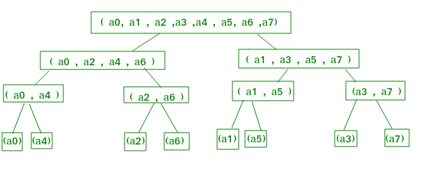
Here is the Divide-and-conquer strategy to solve this problem.
Define two new polynomials of degree-bound n/2, using even-index and odd-index coefficients of A(x) separately



The problem of evaluating A(x) at reduces to evaluating the degree-bound n/2 polynomials A0(x) and A1(x) at the points 

Now combining the results by 

The list does not contain n distinct values, but n/2 complex n/2th roots of unity. Polynomials A0 and A1 are recursively evaluated at the n complex nth roots of unity. Subproblems have exactly the same form as the original problem, but are half the size. So recurrence formed is T(n) = 2T(n/2) + O(n), i.e complexity O(nlogn).

Algorithm
1. Add n higher-order zero coefficients to A(x) and B(x)
2. Evaluate A(x) and B(x) using FFT for 2n points
3. Pointwise multiplication of point-value forms
4. Interpolate C(x) using FFT to compute inverse DFT

Pseudo code of recursive FFT

Recursive_FFT(a){
n = length(a) // a is the input coefficient vector
if n = 1
 then return a

// wn is principle complex nth root of unity.
wn = e^(2*pi*i/n)
w = 1

// even indexed coefficients
A0 = (a0, a2, ..., an-2 )

// odd indexed coefficients
A1 = (a1, a3, ..., an-1 ) 

y0 = Recursive_FFT(A0) // local array
y1 = Recursive-FFT(A1) // local array

for k = 0 to n/2 - 1

 // y array stores values of the DFT 
 // of given polynomial. 
 do y[k] = y0[k] + w*y1[k] 
 y[k+(n/2)] = y0[k] - w*y1[k]
 w = w*wn
return y
}
Recursion Tree of Above Execution-

👁 Fast Fourier Transformation for polynomial multiplication

Why does this work?

since, 
Thus, the vector y returned by Recursive-FFT is indeed the DFT of the input
vector a.

Input: 1 2 3 4
Output:
(10, 0)
(-2, 2)
(-2, 0)
(-2,-2)

Interpolation 
Switch the roles of a and y.
Replace wn by wn^-1.
Divide each element of the result by n.
Time Complexity: O(nlogn).