 |
VOOZH | about |
|
VOOZH | about |
The RIGHT function in Google Sheets is a tool that extracts a specified number of characters from the end of a text string. It's perfect for tasks like isolating suffixes, extracting the last digits of IDs, or organizing structured data.
The RIGHT function operates by counting characters from the end of a text string and returning only the portion you specify.
1. Extracting Suffixes:
RIGHT to pull out file extensions (e.g., .pdf or .docx) or name suffixes (e.g., "Jr." or "III").=RIGHT(A1, 3) extracts the last three characters from the text in cell A1.2. Isolating Specific Digits:
=RIGHT("123456789", 4) returns 6789.3. Cleaning and Formatting Text Data:
=RIGHT(A1, 4) extracts "2023".The RIGHT function simplifies text manipulation in Google Sheets, making it useful for a variety of data management tasks.
=RIGHT(text, [num_chars])
Parameters:
Learn how to easily extract characters from the end of text with the RIGHT function in Google Sheets.
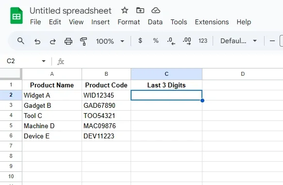
Create a table with sample data and select a cell to enter the formula.
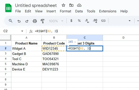
In a new column (e.g., Column C), use the RIGHT function to extract the last 3 digits of the Product Code. Enter the formula in cell C2:
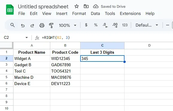
=RIGHT(B2, 3)
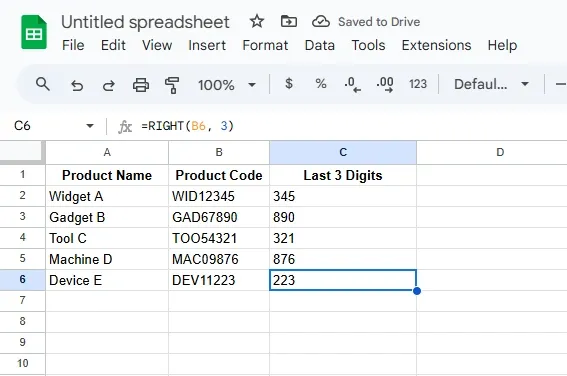
Click and drag the fill handle (bottom-right corner of C2) to apply the formula to the rest of the rows.
The new column will display the last 3 characters of each Product Code:
The RIGHT function can be combined with other Google Sheets functions to perform advanced text manipulations and extractions. Here are some practical examples:
Combine extracted text with another string or value.
=CONCATENATE(RIGHT(A1, 2), B1)
A1 and combine them with the value in B1.Dynamically extract characters by using the length of the string.
=RIGHT(A1, LEN(A1)-3)
A1 except the first three.Extract text after a specific delimiter like a dash (-).
=RIGHT(A1, LEN(A1)-FIND("-", A1))
-) in A1.By combining the RIGHT function with other functions like CONCATENATE, LEN, and FIND, you can create flexible formulas for text manipulation and data cleaning.
The RIGHT function becomes even more powerful when applied in advanced scenarios for dynamic text extraction and data cleaning. Here’s how you can use it:
=ARRAYFORMULA(RIGHT(A1:A10, 3))
A1:A10..csv or .jpg from a list of filenames.=RIGHT(A1, LEN(A1)-3)
A1.These advanced use cases make the RIGHT function a versatile tool for dynamic data extraction and efficient data cleaning, especially when working with large datasets in Google Sheets.
| Error | Cause | Solution |
|---|---|---|
| Incorrect Output for Numbers | Numbers are treated as numeric values instead of text. | Format numbers as text before applying the RIGHT function. Use TEXT(A1, "0") if necessary. |
| Output Includes Unwanted Characters | Data contains extra spaces or unwanted symbols. | Use functions like TRIM to remove spaces or SUBSTITUTE to replace unwanted characters. Example: =TRIM(SUBSTITUTE(A1, "-", "")). |
| #VALUE! Error | Argument is not valid or contains blank cells. | Ensure the referenced cell is not empty and contains valid text or numeric data. |
| Mismatched Length in Output | Trying to extract more characters than available. | Double-check the number of characters specified in the RIGHT function. Use LEN(A1) to confirm string length. |
By addressing these common errors, you can ensure accurate results when using the RIGHT function in Google Sheets.
Also Read: