Essentials of Deep Learning: Visualizing Convolutional Neural Networks in Python

9 min read

Introduction

One of the most debated topics in deep learning is how to interpret and understand a trained model – particularly in the context of high risk industries like healthcare. The term “black box” has often been associated with deep learning algorithms. How can we trust the results of a model if we can’t explain how it works? It’s a legitimate question.

Take the example of a deep learning model trained for detecting cancerous tumours. The model tells you that it is 99% sure that it has detected cancer – but it does not tell you why or how it made that decision.

Did it find an important clue in the MRI scan? Or was it just a smudge on the scan that was incorrectly detected as a tumour? This is a matter of life and death for the patient and doctors cannot afford to be wrong.

👁 Image

In this article, we will explore how to visualize a convolutional neural network (CNN), a deep learning architecture particularly used in most state-of-the-art image based applications. We will get to know the importance of visualizing a CNN model, and the methods to visualize them. We will also take a look at a use case that will help you understand the concept better.

Note: This article assumes that you know the basics of Deep Learning and have previously worked on image processing problems using CNN. Also, we will be using Keras as our deep learning library. If you want to brush up on the concepts, you can go through these articles first:

• Fundamentals of Deep Learning – Starting with Artificial Neural Network
• Architecture of Convolutional Neural Networks (CNNs) demystified
• Tutorial: Optimizing Neural Networks using Keras (with Image recognition case study)

You can also enroll in this free course on CNN to learn about them in structured manner: Convolutional Neural Networks (CNN) from Scratch

Let’s get on with it!

Table of Contents

• Importance of Visualizing a CNN model
• Methods of Visualization
  1. Preliminary Methods
     • Plot Model Architecture
     • Visualize Filters
  2. Activation based Methods
     • Maximal Activation
     • Image Occlusion
  3. Gradient based Methods
     • Saliency Map
     • Gradient based Class Activation Map

Importance of Visualizing a CNN model

As we have seen in the cancerous tumour example above, it is absolutely crucial that we know what our model is doing – and how it’s making decisions on its predictions. Typically, the reasons listed below are the most important points for a deep learning practitioner to remember:

1. Understanding how the model works
2. Assistance in Hyperparameter tuning
3. Finding out the failures of the model and getting an intuition of why they fail
4. Explaining the decisions to a consumer / end-user or a business executive

Let us look at an example where visualizing a neural network model helped in understanding the follies and improving the performance (the below example has been sourced from: http://intelligence.org/files/AIPosNegFactor.pdf).

Once upon a time, the US Army wanted to use neural networks to automatically detect camouflaged enemy tanks. The researchers trained a neural net on 50 photos of camouflaged tanks in trees, and 50 photos of trees without tanks. Using standard techniques for supervised learning, the researchers trained the neural network to a weighting that correctly loaded the training set—output “yes” for the 50 photos of camouflaged tanks, and output “no” for the 50 photos of forest.

This did not ensure, or even imply, that new examples would be classified correctly. The neural network might have “learned” 100 special cases that would not generalize to any new problem. Wisely, the researchers had originally taken 200 photos, 100 photos of tanks and 100 photos of trees. They had used only 50 of each for the training set. The researchers ran the neural network on the remaining 100 photos, and without further training the neural network classified all remaining photos correctly. Success confirmed! The researchers handed the finished work to the Pentagon, which soon handed it back, complaining that in their own tests the neural network did no better than chance at discriminating photos.

👁 Image

It turned out that in the researchers’ dataset, photos of camouflaged tanks had been taken on cloudy days, while photos of plain forest had been taken on sunny days. The neural network had learned to distinguish cloudy days from sunny days, instead of distinguishing camouflaged tanks from an empty forest.

Methods of Visualizing a CNN model

Broadly the methods of Visualizing a CNN model can be categorized into three parts based on their internal workings

• Preliminary methods – Simple methods which show us the overall structure of a trained model
• Activation based methods – In these methods, we decipher the activations of the individual neurons or a group of neurons to get an intuition of what they are doing
• Gradient based methods – These methods tend to manipulate the gradients that are formed from a forward and backward pass while training a model

We will look at each of them in detail in the sections below. Here we will be using keras as our library for building deep learning models and keras-vis for visualizing them. Make sure you have installed these in your system before going ahead.

NOTE: This article uses the dataset given in “Identify the Digits” competition. To run the code mentioned below, you would have to download it in your system. Also, please perform the steps provided in this page before starting with the implementation below.

1. Preliminary Methods

1.1 Plotting model architecture

The simplest thing you can do is to print/plot the model. Here, you can also print the shapes of individual layers of neural network and the parameters in each layer.

In keras, you can implement it as below:

model.summary()

_________________________________________________________________
Layer (type) Output Shape Param # 
=================================================================
conv2d_1 (Conv2D) (None, 26, 26, 32) 320 
_________________________________________________________________
conv2d_2 (Conv2D) (None, 24, 24, 64) 18496 
_________________________________________________________________
max_pooling2d_1 (MaxPooling2 (None, 12, 12, 64) 0 
_________________________________________________________________
dropout_1 (Dropout) (None, 12, 12, 64) 0 
_________________________________________________________________
flatten_1 (Flatten) (None, 9216) 0 
_________________________________________________________________
dense_1 (Dense) (None, 128) 1179776 
_________________________________________________________________
dropout_2 (Dropout) (None, 128) 0 
_________________________________________________________________
preds (Dense) (None, 10) 1290 
=================================================================
Total params: 1,199,882
Trainable params: 1,199,882
Non-trainable params: 0

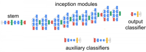
For a more creative and expressive way – you can draw a diagram of the architecture (hint – take a look at the keras.utils.vis_utils function).

👁 Image

1.2 Visualize filters

Another way is to plot the filters of a trained model, so that we can understand the behaviour of those filters. For example, the first filter of the first layer of the above model looks like:

top_layer = model.layers[0]
plt.imshow(top_layer.get_weights()[0][:, :, :, 0].squeeze(), cmap='gray')

👁 Image

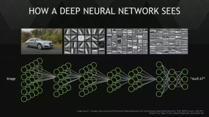
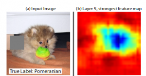
Generally, we see that the low level filters work as edge detectors, and as we go higher, they tend to capture high level concepts like objects and faces.

👁 Image

Source : http://web.eecs.umich.edu/~honglak/cacm2011-researchHighlights-convDBN.pdf

2. Activation Maps

2.1 Maximal Activations

To see what our neural network is doing, we can apply the filters over an input image and then plot the output. This allows us to understand what sort of input patterns activate a particular filter. For example, there could be a face filter that activates when it gets the presence of a face in the image.

from vis.visualization import visualize_activation
from vis.utils import utils
from keras import activations

from matplotlib import pyplot as plt
%matplotlib inline
plt.rcParams['figure.figsize'] = (18, 6)

# Utility to search for layer index by name.
# Alternatively we can specify this as -1 since it corresponds to the last layer.
layer_idx = utils.find_layer_idx(model, 'preds')

# Swap softmax with linear
model.layers[layer_idx].activation = activations.linear
model = utils.apply_modifications(model)

# This is the output node we want to maximize.
filter_idx = 0
img = visualize_activation(model, layer_idx, filter_indices=filter_idx)
plt.imshow(img[..., 0])

👁 Image

We can transfer this idea to all the classes and check how each of them would look like.

PS: Run the script below to check it out.

for output_idx in np.arange(10):
 # Lets turn off verbose output this time to avoid clutter and just see the output.
 img = visualize_activation(model, layer_idx, filter_indices=output_idx, input_range=(0., 1.))
 plt.figure()
 plt.title('Networks perception of {}'.format(output_idx))
 plt.imshow(img[..., 0])

2.2 Image Occlusion

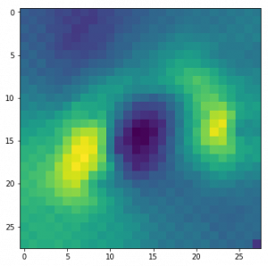
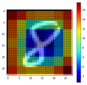
In an image classification problem, a natural question is if the model is truly identifying the location of the object in the image, or just using the surrounding context. We took a brief look at this in gradient based methods above. Occlusion based methods attempt to answer this question by systematically occluding different portions of the input image with a grey square, and monitoring the output of the classifier. The examples clearly show the model is localizing the objects within the scene, as the probability of the correct class drops significantly when the object is occluded.

👁 Image

To understand this concept, let us take a random image from our dataset and try to plot a heatmap of the image. This will give us an intuition of which parts of the image are important for that model in order to make a clear distinction of the actual class.

def iter_occlusion(image, size=8):
 # taken from https://www.kaggle.com/blargl/simple-occlusion-and-saliency-maps

 occlusion = np.full((size * 5, size * 5, 1), [0.5], np.float32)
 occlusion_center = np.full((size, size, 1), [0.5], np.float32)
 occlusion_padding = size * 2

 # print('padding...')
 image_padded = np.pad(image, ( \
 (occlusion_padding, occlusion_padding), (occlusion_padding, occlusion_padding), (0, 0) \
 ), 'constant', constant_values = 0.0)

 for y in range(occlusion_padding, image.shape[0] + occlusion_padding, size):

 for x in range(occlusion_padding, image.shape[1] + occlusion_padding, size):
 tmp = image_padded.copy()

 tmp[y - occlusion_padding:y + occlusion_center.shape[0] + occlusion_padding, \
 x - occlusion_padding:x + occlusion_center.shape[1] + occlusion_padding] \
 = occlusion

 tmp[y:y + occlusion_center.shape[0], x:x + occlusion_center.shape[1]] = occlusion_center

 yield x - occlusion_padding, y - occlusion_padding, \
 tmp[occlusion_padding:tmp.shape[0] - occlusion_padding, occlusion_padding:tmp.shape[1] - occlusion_padding]

i = 23 # for example
data = val_x[i]
correct_class = np.argmax(val_y[i])

# input tensor for model.predict
inp = data.reshape(1, 28, 28, 1)

# image data for matplotlib's imshow
img = data.reshape(28, 28)

# occlusion
img_size = img.shape[0]
occlusion_size = 4

print('occluding...')

heatmap = np.zeros((img_size, img_size), np.float32)
class_pixels = np.zeros((img_size, img_size), np.int16)

from collections import defaultdict
counters = defaultdict(int)

for n, (x, y, img_float) in enumerate(iter_occlusion(data, size=occlusion_size)):

 X = img_float.reshape(1, 28, 28, 1)
 out = model.predict(X)
 #print('#{}: {} @ {} (correct class: {})'.format(n, np.argmax(out), np.amax(out), out[0][correct_class]))
 #print('x {} - {} | y {} - {}'.format(x, x + occlusion_size, y, y + occlusion_size))

 heatmap[y:y + occlusion_size, x:x + occlusion_size] = out[0][correct_class]
 class_pixels[y:y + occlusion_size, x:x + occlusion_size] = np.argmax(out)
 counters[np.argmax(out)] += 1

👁 Image

3. Gradient Based Methods

3.1 Saliency Maps

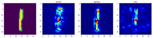
As we saw in the example of tanks, how can we get to know which part does our model focuses on to get prediction? For this, we can use saliency maps. Saliency maps was first introduced in the paper: Deep Inside Convolutional Networks: Visualising Image Classification Models and Saliency Maps.

The concept of using saliency maps is pretty straight-forward – we compute the gradient of the output category with respect to the input image. This should tell us how the output category value changes with respect to a small change in the input image pixels. All the positive values in the gradients tell us that a small change to that pixel will increase the output value. Hence, visualizing these gradients, which are the same shape as the image, should provide some intuition of attention.

Intuitively this method highlights the salient image regions that contribute the most towards the output.

class_idx = 0
indices = np.where(val_y[:, class_idx] == 1.)[0]

# pick some random input from here.
idx = indices[0]

# Lets sanity check the picked image.
from matplotlib import pyplot as plt
%matplotlib inline
plt.rcParams['figure.figsize'] = (18, 6)

plt.imshow(val_x[idx][..., 0])


from vis.visualization import visualize_saliency
from vis.utils import utils
from keras import activations

# Utility to search for layer index by name. 
# Alternatively we can specify this as -1 since it corresponds to the last layer.
layer_idx = utils.find_layer_idx(model, 'preds')

# Swap softmax with linear
model.layers[layer_idx].activation = activations.linear
model = utils.apply_modifications(model)

grads = visualize_saliency(model, layer_idx, filter_indices=class_idx, seed_input=val_x[idx])
# Plot with 'jet' colormap to visualize as a heatmap.
plt.imshow(grads, cmap='jet')


# This corresponds to the Dense linear layer.
for class_idx in np.arange(10): 
 indices = np.where(val_y[:, class_idx] == 1.)[0]
 idx = indices[0]

 f, ax = plt.subplots(1, 4)
 ax[0].imshow(val_x[idx][..., 0])
 
 for i, modifier in enumerate([None, 'guided', 'relu']):
 grads = visualize_saliency(model, layer_idx, filter_indices=class_idx, 
 seed_input=val_x[idx], backprop_modifier=modifier)
 if modifier is None:
 modifier = 'vanilla'
 ax[i+1].set_title(modifier) 
 ax[i+1].imshow(grads, cmap='jet')

👁 Image

3.2 Gradient based Class Activations Maps

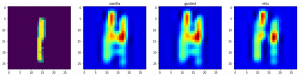
Class activation maps, or grad-CAM, is another way of visualizing what our model looks at while making predictions. Instead of using gradients with respect to the output, grad-CAM uses penultimate Convolutional layer output. This is done to utilize the spacial information that is being stored in the penultimate layer.

from vis.visualization import visualize_cam

# This corresponds to the Dense linear layer.
for class_idx in np.arange(10): 
 indices = np.where(val_y[:, class_idx] == 1.)[0]
 idx = indices[0]

f, ax = plt.subplots(1, 4)
 ax[0].imshow(val_x[idx][..., 0])
 
for i, modifier in enumerate([None, 'guided', 'relu']):
 grads = visualize_cam(model, layer_idx, filter_indices=class_idx, 
 seed_input=val_x[idx], backprop_modifier=modifier) 
 if modifier is None:
 modifier = 'vanilla'
 ax[i+1].set_title(modifier) 
 ax[i+1].imshow(grads, cmap='jet')

👁 Image

End Notes

In this article, we have covered how to visualize a CNN model, and why should you do it along with an example. It has wide ranging applications from helping in medical cases to solving logistical issues for the army.

I hope this will give you an intuition of how to build better models in your own deep learning applications.

If you have any ideas / suggestions regarding the topic, do let me know in the comments below!

Participate in our Hackathons, including the DataHack Premier League and Lord of the Machines!

Login to continue reading and enjoy expert-curated content.

Free Courses

Become an Author

Share insights, grow your voice, and inspire the data community.

• Reach a Global Audience
• Share Your Expertise with the World
• Build Your Brand & Audience

• Join a Thriving AI Community
• Level Up Your AI Game
• Expand Your Influence in Genrative AI

👁 imag