Architecture of Convolutional Neural Networks (CNNs) demystified

14 min read

Introduction

I will start with a confession – there was a time when I didn’t really understand deep learning. I would look at the research papers and articles on the topic and feel like it is a very complex topic. I tried understanding Neural networks and their various types, but it still looked difficult.

Then one day, I decided to take one step at a time. I decided to start with basics and build on them. I decided that I will break down the steps applied in these techniques and do the steps (and calculations) manually, until I understand how they work. It was time taking and intense effort – but the results were phenomenal.

Now, I can not only understand the spectrum of deep learning, I can visualize things and come up with better ways because my fundamentals are clear. It is one thing to apply neural networks mindlessly and it is other to understand what is going on and how are things happening at the back.

Today, I am going to share this secret recipe with you. I will show you how I took the Convolutional Neural Networks and worked on them till I understood them. I will walk you through the journey so that you develop a deep understanding of how CNNs work.

If you would like to learn the architecture and working of CNN in a course format, you can enrol in this free course too: Convolutional Neural Networks from Scratch

In this article I am going to discuss the architecture behind Convolutional Neural Networks, which are designed to address image recognition and classification problems.

I am assuming that you have a basic understanding of how a neural network works. If you’re not sure of your understanding I would request you to go through this article before you read on.

Table of Contents:

1. How does a machine look at an image?
2. How do we help a neural network to identify images?
3. Defining a Convolutional neural network
   1. Convolution Layer
   2. Pooling Layer
   3. Output Layer
4. Putting it all together
5. Using CNN to classify images

1. How does a machine look at an image?

Human brain is a very powerful machine. We see (capture) multiple images every second and process them without realizing how the processing is done. But, that is not the case with machines. The first step in image processing is to understand, how to represent an image so that the machine can read it?

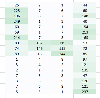
In simple terms, every image is an arrangement of dots (a pixel) arranged in a special order. If you change the order or color of a pixel, the image would change as well. Let us take an example. Let us say, you wanted to store and read an image with a number 4 written on it.

The machine will basically break this image into a matrix of pixels and store the color code for each pixel at the representative location. In the representation below – number 1 is white and 256 is the darkest shade of green color (I have constrained the example to have only one color for simplicity).

👁 Image

Once you have stored the images in this format, the next challenge is to have our neural network understand the arrangement and the pattern.

2. How do we help a neural network to identify images?

A number is formed by having pixels arranged in a certain fashion.

👁 Image

Let’s say we try to use a fully connected network to identify it? What does it do?

A fully connected network would take this image as an array by flattening it and considering pixel values as features to predict the number in image. Definitely it’s tough for the network to understand what’s happening underneath.

👁 Image

It’s impossible even for a human to identify that this is a representation of number 4. We have lost the spatial arrangement of pixels completely.

What can we possibly do? Let’s try to extract features from the original image such that the spatial arrangement is preserved.

 Case 1:

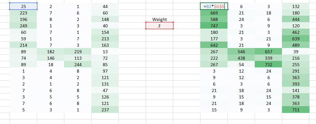
Here we have used a weight to multiply the initial pixel values.

👁 Image

It does get easier for the naked eye to identify that this is a 4. But again to send this image to a fully connected network, we would have to flatten it. We are unable to preserve the spatial arrangement of the image.

👁 Image

Case 2:

Now we can see that flattening the image destroys its arrangement completely. we need to devise a way to send images to a network without flattening them and retaining its spatial arrangement. We need to send 2D/3D arrangement of pixel values.

Let’s try taking two pixel values of the image at a time rather than taking just one. This would give the network a very good insight as to how does the adjacent pixel look like. Now that we’re taking two pixels at a time, we shall take two weight values too.

👁 Image

I hope you noted that the image now became a 3 column arrangement from a 4 column arrangement initially. The image got smaller since we’re now moving two pixels at a time (pixels are getting shared in each movement). We made the image smaller and we can still understand that it’s a 4 to quite a great extent. Also, an important fact to realise is that we we’re taking two consecutive horizontal pixels, therefore only horizontal arrangement is considered here.

This is one way to extract features from an image. We’re able to see the left and middle part well, however the right side is not so clear. This is because of the following two problems-

1. The left and right corners of the image is multiplied by the weights just once.
2. The left part is still retained since the weight value is high while the right part is getting slightly lost due to low weight value.

Now we have two problems, we shall have two solutions to solve them as well.

Case 3:

The problem encountered is that the left and right corners of the image is getting passed by the weight just once. What we need to do is we need the network to consider the corners also like other pixels.

We have a simple solution to solve this. Put zeros along the sides of the weight movement.

👁 Image

You can see that by adding the zeroes the information from the corners is retained. The size of the image is higher too. This can be used in cases where we don’t want the image size to reduce.

Case 4:

The problem we’re trying to address here is that a smaller weight value in the right side corner is reducing the pixel value thereby making it tough for us to recognize. What we can do is, we take multiple weight values in a single turn and put them together.

A weight value of (1,0.3) gave us an output of the form

👁 Image

while a weight value of the form (0.1,5) would give us an output of the form

👁 Image

A combined version of these two images would give us a very clear picture. Therefore what we did was simply use multiple weights rather than just one to retain more information about the image. The final output would be a combined version of the above two images.

Case 5:

Till now we have used the weights which were trying to take horizontal pixels together. But in most cases we need to preserve the spatial arrangement in both horizontal and vertical direction. We can take the weight as a 2D matrix which takes pixels together in both horizontal and vertical direction. Also, keep in mind that since we have taken both horizontal and vertical movement of weights, the output is one pixel lower in both horizontal and vertical direction.👁 Image

Special thanks to Jeremy Howard for the inspiring me to create these visuals.

So what did we do?

What we did above was that we were trying to extract features from an image by using the spatial arrangement of the images. To understand an image its extremely important for a network to understand how the pixels are arranged. What we did above is what exactly a convolutional neural network does. We can take the input image, define a weight matrix and the input is convolved to extract specific features from the image without losing the information about its spatial arrangement.

Another great benefit this approach has is that it reduces the number of parameters from the image. As you saw above the convolved images had lesser pixels as compared to the original image. This dramatically reduces the number of parameters we need to train for the network.

3. Defining a Convolutional Neural Network

We need three basic components to define a basic convolutional network.

1. The convolutional layer
2. The Pooling layer[optional]
3. The output layer

Let’s see each of these in a little more detail

2.1 The Convolution Layer

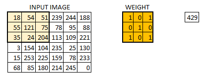
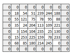
In this layer, what happens is exactly what we saw in case 5 above. Suppose we have an image of size 6*6. We define a weight matrix which extracts certain features from the images

👁 Image

We have initialized the weight as a 3*3 matrix. This weight shall now run across the image such that all the pixels are covered at least once, to give a convolved output. The value 429 above, is obtained by the adding the values obtained by element wise multiplication of the weight matrix and the highlighted 3*3 part of the input image.

👁 Image

The 6*6 image is now converted into a 4*4 image.  Think of weight matrix like a paint brush painting a wall. The brush first paints the wall horizontally and then comes down and paints the next row horizontally. Pixel values are used again when the weight matrix moves along the image. This basically enables parameter sharing in a convolutional neural network.

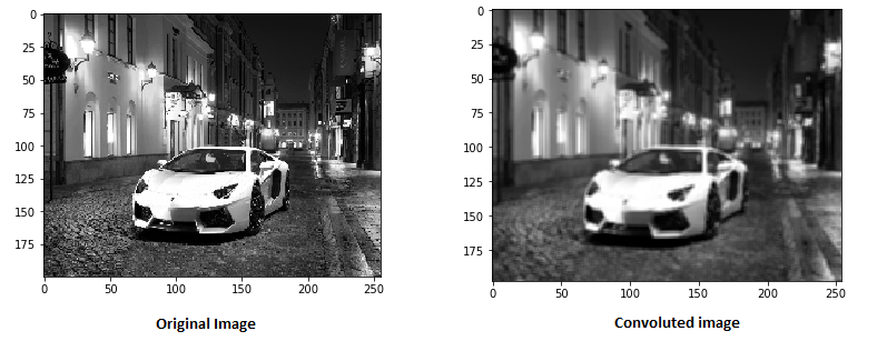
Let’s see how this looks like in a real image.

👁 Image

The weight matrix behaves like a filter in an image extracting particular information from the original image matrix. A weight combination might be extracting edges, while another one might a particular color, while another one might just blur the unwanted noise.

The weights are learnt such that the loss function is minimized similar to an MLP. Therefore weights are learnt to extract features from the original image which help the network in correct prediction. When we have multiple convolutional layers, the initial layer extract more generic features, while as the network gets deeper, the features extracted by the weight matrices are more and more complex and more suited to the problem at hand.

The concept of stride and padding

As we saw above, the filter or the weight matrix, was moving across the entire image moving one pixel at a time. We can define it like a hyperparameter, as to how we would want the weight matrix to move across the image. If the weight matrix moves 1 pixel at a time, we call it as a stride of 1. Let’s see how a stride of 2 would look like.

👁 Image

As you can see the size of image keeps on reducing as we increase the stride value. Padding the input image with zeros across it solves this problem for us. We can also add more than one layer of zeros around the image in case of higher stride values.

👁 Image

We can see how the initial shape of the image is retained after we padded the image with a zero. This is known as same padding since the output image has the same size as the input. 👁 Image

This is known as same padding (which means that we considered only the valid pixels of the input image). The middle 4*4 pixels would be the same. Here we have retained more information from the borders and have also preserved the size of the image.

Multiple filters and the activation map

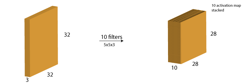
One thing to keep in mind is that the depth dimension of the weight would be same as the depth dimension of the input image. The weight extends to the entire depth of the input image. Therefore, convolution with a single weight matrix would result into a convolved output with a single depth dimension. In most cases instead of a single filter(weight matrix), we have multiple filters of the same dimensions applied together.

The output from the each filter is stacked together forming the depth dimension of the convolved image. Suppose we have an input image of size 32*32*3. And we apply 10 filters of size 5*5*3 with valid padding. The output would have the dimensions as 28*28*10.

You can visualize it as –

👁 Image

This activation map is the output of the convolution layer.

2.2 The Pooling Layer

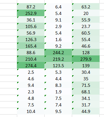
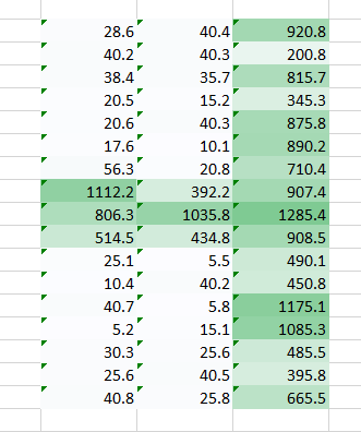
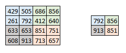
Sometimes when the images are too large, we would need to reduce the number of trainable parameters. It is then desired to periodically introduce pooling layers between subsequent convolution layers. Pooling is done for the sole purpose of reducing the spatial size of the image. Pooling is done independently on each depth dimension, therefore the depth of the image remains unchanged. The most common form of pooling layer generally applied is the max pooling.

👁 Image

Here we have taken stride as 2, while pooling size also as 2. The max operation is applied to each depth dimension of the convolved output. As you can see, the 4*4 convolved output has become 2*2 after the max pooling operation.

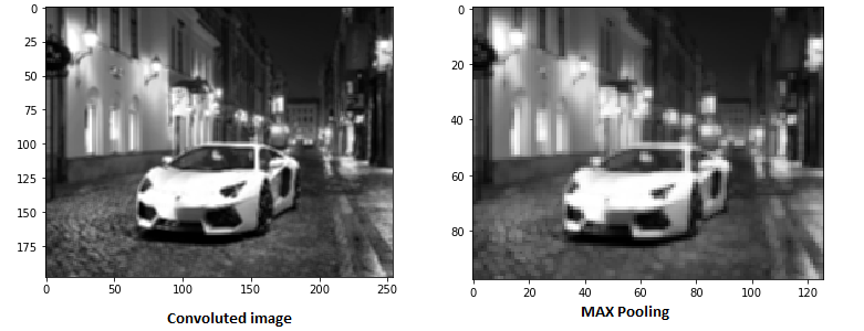
Let’s see how max pooling looks on a real image.

👁 Image

As you can see I have taken convoluted image and have applied max pooling on it. The max pooled image still retains the information that it’s a car on a street. If you look carefully, the dimensions if the image have been halved. This helps to reduce the parameters to a great extent.

Similarly other forms of pooling can also be applied like average pooling or the L2 norm pooling.

Output dimensions

It might be getting a little confusing for you to understand the input and output dimensions at the end of each convolution layer. I decided to take these few lines to make you capable of identifying the output dimensions. Three hyperparameter would control the size of output volume.

1. The number of filters – the depth of the output volume will be equal to the number of filter applied. Remember how we had stacked the output from each filter to form an activation map. The depth of the activation map will be equal to the number of filters.
2. Stride – When we have a stride of one we move across and down a single pixel. With higher stride values, we move large number of pixels at a time and hence produce smaller output volumes.
3. Zero padding – This helps us to preserve the size of the input image. If a single zero padding is added, a single stride filter movement would retain the size of the original image.

We can apply a simple formula to calculate the output dimensions. The spatial size of the output image can be calculated as( [W-F+2P]/S)+1. Here, W is the input volume size, F is the size of the filter, P is the number of padding applied and S is the number of strides. Suppose we have an input image of size 32*32*3, we apply 10 filters of size 3*3*3, with single stride and no zero padding.

Here W=32, F=3, P=0 and S=1. The output depth will be equal to the number of filters applied i.e. 10.

The size of the output volume will be ([32-3+0]/1)+1 = 30. Therefore the output volume will be 30*30*10.

2.3 The Output layer

After multiple layers of convolution and padding, we would need the output in the form of a class. The convolution and pooling layers would only be able to extract features and reduce the number of parameters from the original images. However, to generate the final output we need to apply a fully connected layer to generate an output equal to the number of classes we need. It becomes tough to reach that number with just the convolution layers. Convolution layers generate 3D activation maps while we just need the output as whether or not an image belongs to a particular class. The output layer has a loss function like categorical cross-entropy, to compute the error in prediction. Once the forward pass is complete the backpropagation begins to update the weight and biases for error and loss reduction.

3. Putting it all together – How does the entire network look like?

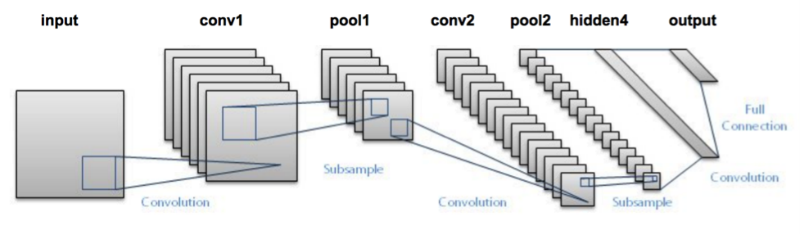
CNN as you can now see is composed of various convolutional and pooling layers. Let’s see how the network looks like.

👁 Image

• We pass an input image to the first convolutional layer. The convoluted output is obtained as an activation map. The filters applied in the convolution layer extract relevant features from the input image to pass further.
• Each filter shall give a different feature to aid the correct class prediction. In case we need to retain the size of the image, we use same padding(zero padding), otherwise valid padding is used since it helps to reduce the number of features.
• Pooling layers are then added to further reduce the number of parameters
• Several convolution and pooling layers are added before the prediction is made. Convolutional layer help in extracting features. As we go deeper in the network more specific features are extracted as compared to a shallow network where the features extracted are more generic.
• The output layer in a CNN as mentioned previously is a fully connected layer, where the input from the other layers is flattened and sent so as the transform the output into the number of classes as desired by the network.
• The output is then generated through the output layer and is compared to the output layer for error generation. A loss function is defined in the fully connected output layer to compute the mean square loss. The gradient of error is then calculated.
• The error is then backpropagated to update the filter(weights) and bias values.
• One training cycle is completed in a single forward and backward pass.

4. Using CNN to classify images in KERAS

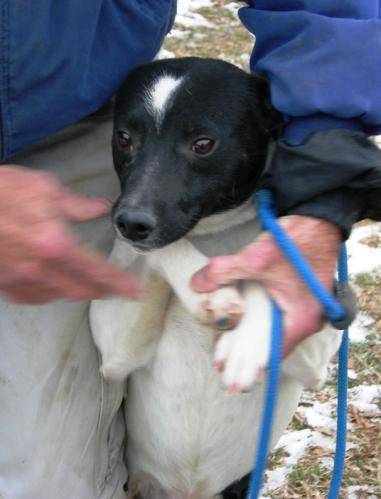
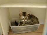
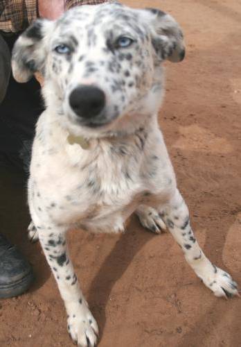
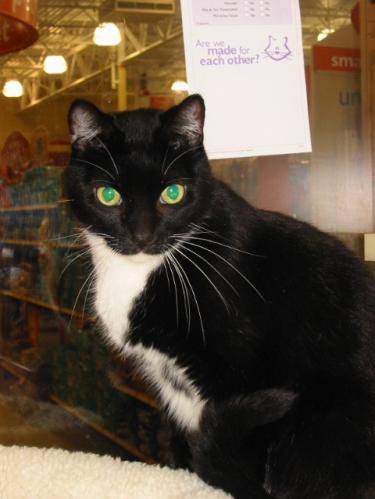
Let’s try taking an example where we input several images of cats and dogs and we try to classify these images into their respective animal category using a CNN. This is a classic problem of image recognition and classification. What the machine needs to do is it needs to see the image and understand by the various features as to whether its a cat or a dog.

The features can be like extracting the edges, or extracting the whiskers of a cat etc. The convolutional layer would extract these features. Let’s take a hand on the data set.

These are the examples of some of the images in the dataset.

👁 Image
👁 Image
👁 Image
👁 Image

We would first need to resize these images to get them all in the same shape. This is something we would generally need to do while handling images, since while capturing images, it would be impossible to capture all images of the same size.

For simplicity of your understanding I have just used a single convolution layer and a single pooling layer, which generally doesn’t happen when we’re trying to make predictions. Dataset used can be downloaded from here.

#import various packages

import os
import numpy as np
import pandas as pd
import scipy
import sklearn
import keras
from keras.models import Sequential
import cv2
from skimage import io
%matplotlib inline

#Defining the File Path

cat=os.listdir("/mnt/hdd/datasets/dogs_cats/train/cat")
dog=os.listdir("/mnt/hdd/datasets/dogs_cats/train/dog")
filepath="/mnt/hdd/datasets/dogs_cats/train/cat/"
filepath2="/mnt/hdd/datasets/dogs_cats/train/dog/"

#Loading the Images

images=[]
label = []
for i in cat:
    image = scipy.misc.imread(filepath+i)
    images.append(image)
    label.append(0) #for cat images

for i in dog:
    image = scipy.misc.imread(filepath2+i)
    images.append(image)
    label.append(1) #for dog images

#resizing all the images

for i in range(0,23000):
    images[i]=cv2.resize(images[i],(300,300))

#converting images to arrays

images=np.array(images)
label=np.array(label)

# Defining the hyperparameters

filters=10
filtersize=(5,5)

epochs =5
batchsize=128

input_shape=(300,300,3)

#Converting the target variable to the required size

from keras.utils.np_utils import to_categorical
label = to_categorical(label)

#Defining the model

model = Sequential()

model.add(keras.layers.InputLayer(input_shape=input_shape))

model.add(keras.layers.convolutional.Conv2D(filters, filtersize, strides=(1, 1), padding='valid', data_format="channels_last", activation='relu'))
model.add(keras.layers.MaxPooling2D(pool_size=(2, 2)))
model.add(keras.layers.Flatten())

model.add(keras.layers.Dense(units=2, input_dim=50,activation='softmax'))

model.compile(loss='categorical_crossentropy', optimizer='adam', metrics=['accuracy'])
model.fit(images, label, epochs=epochs, batch_size=batchsize,validation_split=0.3)

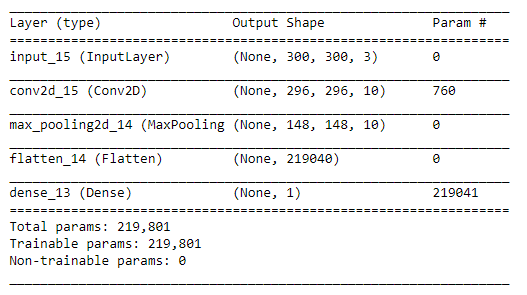
model.summary()

👁 Image

In this model, I have only used a single convolution and Pooling layer and the trainable parameters are 219,801. Wonder how many would I have had if I had used an MLP in this case. You can reduce the number of parameters by further by adding more convolution and pooling layers. The more convolution layers we add the features extracted would be more specific and intricate.

Projects

Now, its time to take the plunge and actually play with some other real datasets. So are you ready to take on the challenge? Accelerate your deep learning journey with the following Practice Problems:

👁 Image	Practice Problem: Identify the Apparels	Identify the type of apparel for given images
👁 Image	Practice Problem: Identify the Digits	Identify the digit in given images

End Notes

I hope through this article I was able to provide you an intuition into convolutional neural networks. I did not go into the complex mathematics of CNN. In case you’re fond of understanding the same – stay tuned, there’s much more lined up for you. Try building your own CNN network to understand how it operates and makes predictions on images. Let me know your findings and approach using the comments section.

Login to continue reading and enjoy expert-curated content.

Free Courses

Become an Author

Share insights, grow your voice, and inspire the data community.

• Reach a Global Audience
• Share Your Expertise with the World
• Build Your Brand & Audience

• Join a Thriving AI Community
• Level Up Your AI Game
• Expand Your Influence in Genrative AI

👁 imag