Tutorial — How to visualize Feature Maps directly from CNN layers

Introduction

Let’s put on the eyes of Neural Networks and see what the Convolution Neural Networks see.

Pre-requisites:-

1. The reader knows how to generate the CNN model.
2. The reader understands the trainable parameter calculations and the size of inputs and outputs of various intermediate layers.

Imp Note:-

1. Here, we are only concerned with building a CNN model and checking its feature maps. We are not concerned about the accuracy of the model.

Now, without wasting our time let us build a model:-

We create a multi-class model with three classes.

model=tf.keras.models.Sequential([
 
 tf.keras.layers.Conv2D(8,(3,3),activation ='relu', input_shape=(150,150,3)),
 tf.keras.layers.MaxPooling2D(2,2),
 
 tf.keras.layers.Conv2D(16,(3,3),activation ='relu'),
 tf.keras.layers.MaxPooling2D(2,2),
 
 tf.keras.layers.Conv2D(32,(3,3),activation ='relu'),
 tf.keras.layers.MaxPooling2D(2,2),
 
 tf.keras.layers.Flatten(),
 
 tf.keras.layers.Dense(1024,activation='relu'),
 tf.keras.layers.Dense(512,activation='relu'),
 
 tf.keras.layers.Dense(3,activation='softmax') 
 ])

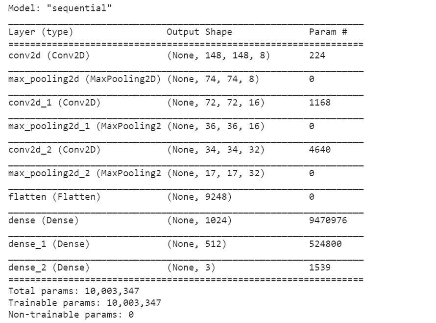
The summary of the model is:-

model.summary()

As we can see above, we have three Convolution Layers followed by MaxPooling Layers, two Dense Layers, and one final output Dense Layer.

Imp note:- We need to compile and fit the model. Hence run the model first, only then we will be able to generate the feature maps. I have not shown all those steps here.

To generate feature maps we need to understand model.layers API.

Accessing Intermediate Layers of CNN:-

Let us understand how to access the intermediate layers of CNN.

Getting names of layers of CNN:-

layer_names = [layer.name for layer in model.layers]
layer_names

Which gives the output as:-

['conv2d',
 'max_pooling2d',
 'conv2d_1',
 'max_pooling2d_1',
 'conv2d_2',
 'max_pooling2d_2',
 'flatten',
 'dense',
 'dense_1',
 'dense_2']

Checking the layers:-

model.layers

It returns the list of Layers as below:-

[<tensorflow.python.keras.layers.convolutional.Conv2D at 0x2510de50e48>,
 <tensorflow.python.keras.layers.pooling.MaxPooling2D at 0x25124b740c8>,
 <tensorflow.python.keras.layers.convolutional.Conv2D at 0x25124b74748>,
 <tensorflow.python.keras.layers.pooling.MaxPooling2D at 0x25124b74d48>,
 <tensorflow.python.keras.layers.convolutional.Conv2D at 0x25124b9e308>,
 <tensorflow.python.keras.layers.pooling.MaxPooling2D at 0x25124b9e988>,
 <tensorflow.python.keras.layers.core.Flatten at 0x25124b9ee88>,
 <tensorflow.python.keras.layers.core.Dense at 0x25124ba13c8>,
 <tensorflow.python.keras.layers.core.Dense at 0x25124ba1988>,
 <tensorflow.python.keras.layers.core.Dense at 0x25124ba1f48>]

Getting output of the layers of CNN:-

layer_outputs = [layer.output for layer in model.layers]

This returns the output objects of the layers. They are not the real output but they tell us the functions which will be generating the outputs. We will be incorporating this layer.output into a visualization model we will build to extract the feature maps.

[<tf.Tensor 'conv2d/Relu:0' shape=(None, 148, 148, 8) dtype=float32>,
 <tf.Tensor 'max_pooling2d/MaxPool:0' shape=(None, 74, 74, 8) dtype=float32>,
 <tf.Tensor 'conv2d_1/Relu:0' shape=(None, 72, 72, 16) dtype=float32>,
 <tf.Tensor 'max_pooling2d_1/MaxPool:0' shape=(None, 36, 36, 16) dtype=float32>,
 <tf.Tensor 'conv2d_2/Relu:0' shape=(None, 34, 34, 32) dtype=float32>,
 <tf.Tensor 'max_pooling2d_2/MaxPool:0' shape=(None, 17, 17, 32) dtype=float32>,
 <tf.Tensor 'flatten/Reshape:0' shape=(None, 9248) dtype=float32>,
 <tf.Tensor 'dense/Relu:0' shape=(None, 1024) dtype=float32>,
 <tf.Tensor 'dense_1/Relu:0' shape=(None, 512) dtype=float32>,
 <tf.Tensor 'dense_2/Softmax:0' shape=(None, 3) dtype=float32>]

To generate feature maps, we have to build a visualization model that takes an image as an input and has the above-mentioned layer_outputs as output functions.

Important thing to note here is that we have total 10 outputs, 9 intermediate outputs and 1 final classification output. Hence, we will have 9 feature maps.

Feature maps visualization Model from CNN Layers

feature_map_model = tf.keras.models.Model(input=model.input, output=layer_outputs)

The above formula just puts together the input and output functions of the CNN model we created at the beginning.

There are a total of 10 output functions in layer_outputs. The image is taken as input and then that image is made to pass through all these 10 output functions one by one in serial order.

The last output function is the output of the model itself. So, in total there are 9 intermediate output functions and hence 9 intermediate feature maps.

This means any input we give to the feature_map_model, the output will be in the form of 9 feature maps.

Now, we will prepare an image to give it as an input to the above feature_map_model:-

image_path= r"path of the image from desktop or internet."img = load_img(image_path, target_size=(150, 150)) input = img_to_array(img) 
input = x.reshape((1,) + x.shape) 
input /= 255.0

In the above code, we have loaded an image into a variable “input”, converted it to an array, expanded the dimensions of the image to match the dimensions of the intermediate layers, and finally, we have scaled the image before feeding it to the layers.

Now, let’s feed it into the model created:-

feature_maps = feature_map_model.predict(input)

The above code has finally generated feature maps for us.

We will again decode the feature_maps content.

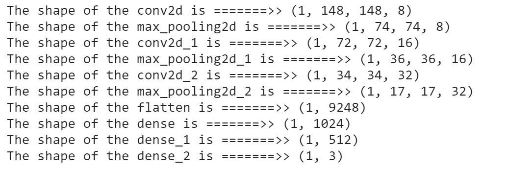
Now that the feature maps are generated, let us check the shape of the feature maps of each of the outputs.

for layer_name, feature_map in zip(layer_names, feature_maps):print(f"The shape of the {layer_name} is =======>> {feature_map.shape}")

The above code will give the layer name of intermediate layers of the CNN Model and the shape of the corresponding feature maps we have generated.

Steps to generate feature maps:-

We need to generate feature maps of only convolution layers and not dense layers and hence we will generate feature maps of layers that have “dimension=4″.

for layer_name, feature_map in zip(layer_names, feature_maps): if len(feature_map.shape) == 4

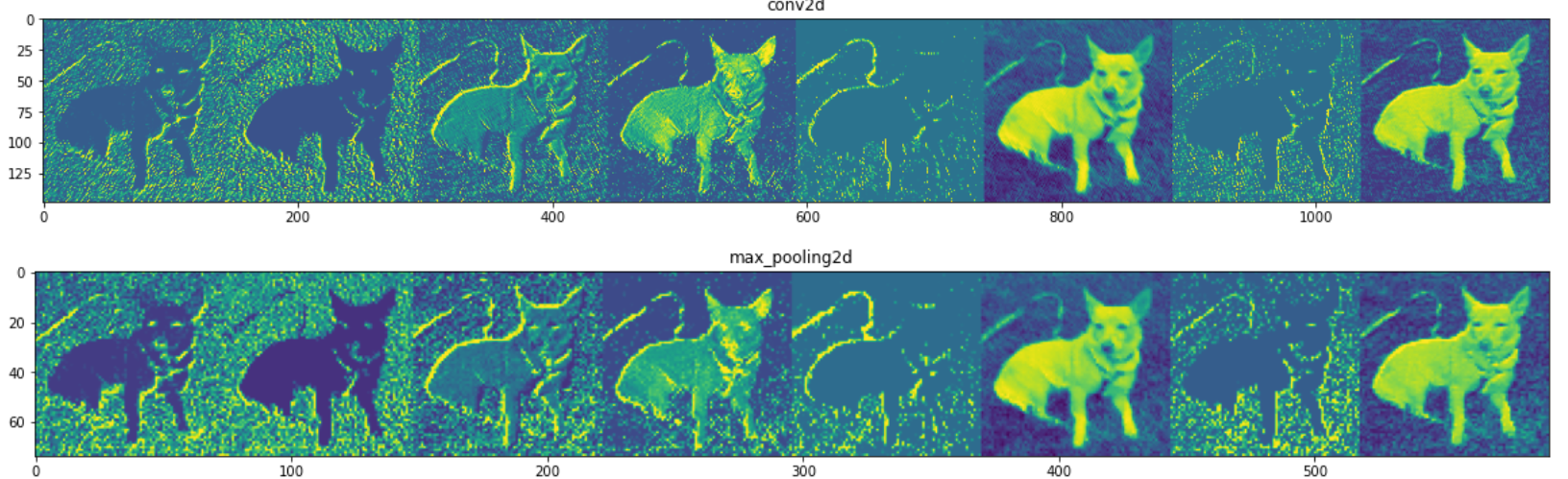
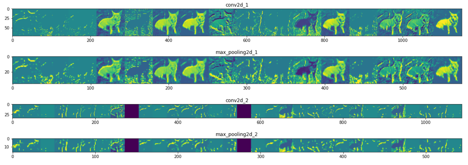
Each feature map has n-channels and this number “n” is given at the end of the shape of the feature map. This is the number of features in a particular layer.

For eg. feature_map[0].shape = (1,148,148,8). This means this is an image with 8 dimensions. So, we need to iterate over this image to separate its 8 images. This shows that layer_1 output has 8 features which have been clubbed into 1 image.

for layer_name, feature_map in zip(layer_names, feature_maps): if len(feature_map.shape) == 4# Number of feature images/dimensions in a feature map of a layer 
  k = feature_map.shape[-1] 
 
 #iterating over a feature map of a particular layer to separate all feature images. for i in range(k):
 feature_image = feature_map[0, :, :, i]

The feature maps directly generated are very dim in visual and hence not properly visible to human eyes. So, we need to do Standardization and Normalization of the feature image extracted.

Standardization and Normalization of an image to make it palatable to human eyes:-

 feature_image-= feature_image.mean()
 feature_image/= feature_image.std ()
 feature_image*= 64
 feature_image+= 128
 feature_image= np.clip(x, 0, 255).astype('uint8')

With keeping the above three points, let us generate feature maps,

for layer_name, feature_map in zip(layer_names, feature_maps): if len(feature_map.shape) == 4
 k = feature_map.shape[-1] 
 size=feature_map.shape[1]
 for i in range(k):
 feature_image = feature_map[0, :, :, i]
 feature_image-= feature_image.mean()
 feature_image/= feature_image.std ()
 feature_image*= 64
 feature_image+= 128
 feature_image= np.clip(x, 0, 255).astype('uint8')
 image_belt[:, i * size : (i + 1) * size] = feature_image

Finally let us display the image_belts we have generated:-

 scale = 20. / k
 plt.figure( figsize=(scale * k, scale) )
 plt.title ( layer_name )
 plt.grid ( False )
 plt.imshow( image_belt, aspect='auto')

Original image — (150,150,3)

Thanks for your time. Kindly, Do give your feedback for the blog.

Hi, Thanks for your code, it is really useful. I want to know what is the 'x' in the image reshpae part input = x.reshape((1,) + x.shape)

Dear Author, Thanks for your writing. I have a query related to the feature map, what happened if the input image is of high resolution? Suppose, you visualize an image with 150 x 150 image if that would be 400 x 400 image then is there any change in feature visualization? Thanks in advance

You use variable "x" without defining it randomly as well as "image_belt" The concepts of the code are clear but the code itself is broken