 |
VOOZH | about |
|
VOOZH | about |
Hello Readers!!
OpenCV – Open Source Computer Vision. It is one of the most widely used tools for computer vision and image processing tasks. It is used in various applications such as face detection, video capturing, tracking moving objects, object disclosure, nowadays in Covid applications such as face mask detection, social distancing, and many more. If you want to know more about OpenCV, check this link.
📌If you want to know about Python Libraries For Image Processing 😋then check this Link.
📌If you want to learn Image processing using NumPy, 😋check this link.
📌For more articles😉, click here
In this blog, I am going to cover OpenCV in great detail by covering some most important tasks in image processing by practical implementation. So let’s get started!!⌛
Image Source
Image Source
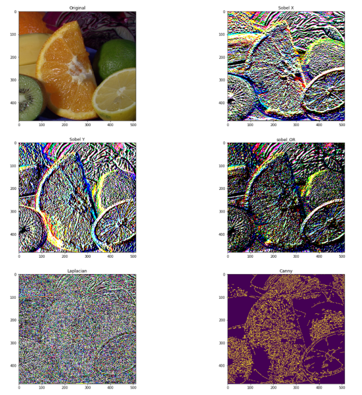
It is one of the most fundamental and important techniques in image processing. Check the below code for complete implementation. For more information, check this link.
image = cv2.imread('fruit.jpg')
image = cv2.cvtColor(image, cv2.COLOR_BGR2RGB)
hgt, wdt,_ = image.shape
# Sobel Edges
x_sobel = cv2.Sobel(image, cv2.CV_64F, 0, 1, ksize=5)
y_sobel = cv2.Sobel(image, cv2.CV_64F, 1, 0, ksize=5)
plt.figure(figsize=(20, 20))
plt.subplot(3, 2, 1)
plt.title("Original")
plt.imshow(image)
plt.subplot(3, 2, 2)
plt.title("Sobel X")
plt.imshow(x_sobel)
plt.subplot(3, 2, 3)
plt.title("Sobel Y")
plt.imshow(y_sobel)
sobel_or = cv2.bitwise_or(x_sobel, y_sobel)
plt.subplot(3, 2, 4)
plt.imshow(sobel_or)
laplacian = cv2.Laplacian(image, cv2.CV_64F)
plt.subplot(3, 2, 5)
plt.title("Laplacian")
plt.imshow(laplacian)
## There are two values: threshold1 and threshold2.
## Those gradients that are greater than threshold2 => considered as an edge
## Those gradients that are below threshold1 => considered not to be an edge.
## Those gradients Values that are in between threshold1 and threshold2 => either classified as edges or non-edges
# The first threshold gradient
canny = cv2.Canny(image, 50, 120)
plt.subplot(3, 2, 6)
plt.imshow(canny)
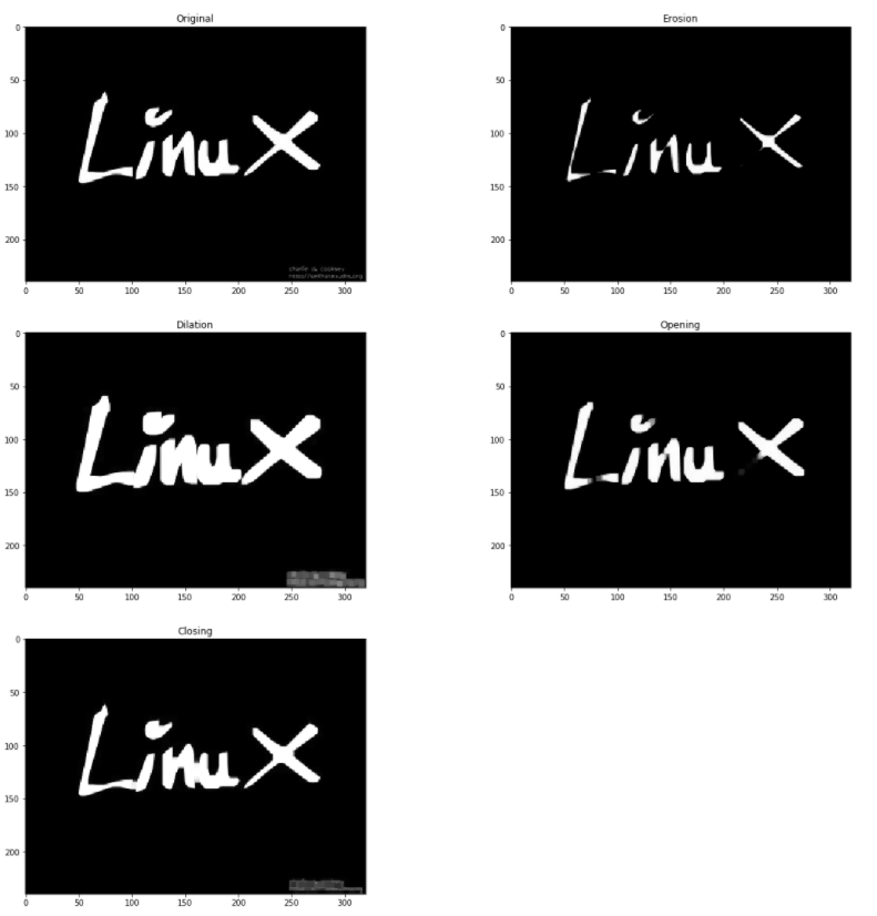
These are two fundamental image processing operations. These are used to removing noises, finding an intensity hole or bump in an image and many more. Check the below code for practical implementation. For more information, check this link.
image = cv2.imread('LinuxLogo.jpg')
image = cv2.cvtColor(image, cv2.COLOR_BGR2RGB)
plt.figure(figsize=(20, 20))
plt.subplot(3, 2, 1)
plt.title("Original")
plt.imshow(image)

kernel = np.ones((5,5), np.uint8)

erosion = cv2.erode(image, kernel, iterations = 1)
plt.subplot(3, 2, 2)
plt.title("Erosion")
plt.imshow(erosion)
dilation = cv2.dilate(image, kernel, iterations = 1)
plt.subplot(3, 2, 3)
plt.title("Dilation")
plt.imshow(dilation)

opening = cv2.morphologyEx(image, cv2.MORPH_OPEN, kernel)
plt.subplot(3, 2, 4)
plt.title("Opening")
plt.imshow(opening)

closing = cv2.morphologyEx(image, cv2.MORPH_CLOSE, kernel)
plt.subplot(3, 2, 5)
plt.title("Closing")
plt.imshow(closing)
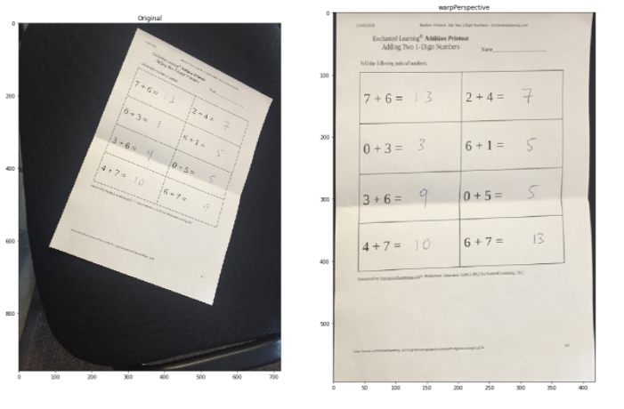
For getting better information about an image, w can change the perspective of a video or an image. In this transformation, we need to provide the points on an image from where we want to take information by changing the perspective. In OpenCV, we use two functions for Perspective transformation getPerspectiveTransform() and then warpPerspective(). Check the below code for complete implementation. For more information, check this link.
image = cv2.imread('scan.jpg')
image = cv2.cvtColor(image, cv2.COLOR_BGR2RGB)
plt.figure(figsize=(20, 20))
plt.subplot(1, 2, 1)
plt.title("Original")
plt.imshow(image)
points_A = np.float32([[320,15], [700,215], [85,610], [530,780]])
points_B = np.float32([[0,0], [420,0], [0,594], [420,594]])
M = cv2.getPerspectiveTransform(points_A, points_B)
warped = cv2.warpPerspective(image, M, (420,594))
plt.subplot(1, 2, 2)
plt.title("warpPerspective")
plt.imshow(warped)
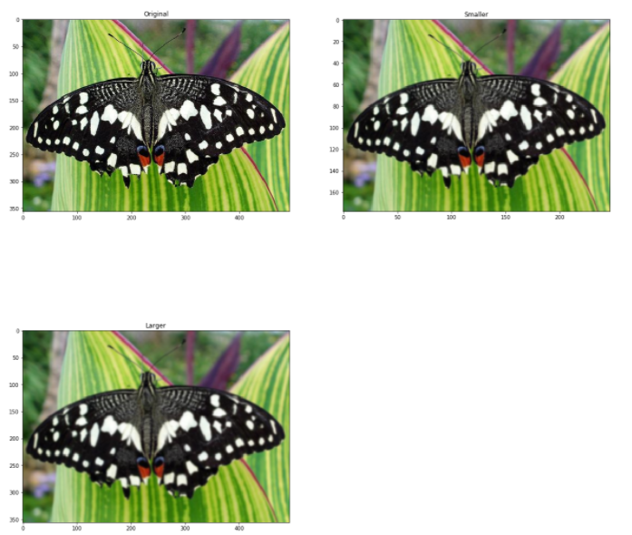
It is a very useful technique when we required scaling in object detection. OpenCV uses two common kinds of image pyramids Gaussian and Laplacian pyramid. Use the pyrUp() and pyrDown() function in OpenCV to downsample or upsample a image. Check the below code for practical implementation. For more information, check this link.
image = cv2.imread('butterfly.jpg')
image = cv2.cvtColor(image, cv2.COLOR_BGR2RGB)
plt.figure(figsize=(20, 20))
plt.subplot(2, 2, 1)
plt.title("Original")
plt.imshow(image)
smaller = cv2.pyrDown(image)
larger = cv2.pyrUp(smaller)
plt.subplot(2, 2, 2)
plt.title("Smaller")
plt.imshow(smaller)
plt.subplot(2, 2, 3)
plt.title("Larger")
plt.imshow(larger)
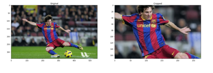
It is one of the most important and fundamental techniques in image processing, Cropping is used to get a particular part of an image. To crop an image. You just need the coordinates from an image according to your area of interest. For a complete analysis, check the below code in OpenCV.
image = cv2.imread('messi.jpg')
image = cv2.cvtColor(image, cv2.COLOR_BGR2RGB)
plt.figure(
Aigsize=(20, 20))
plt.subplot(2, 2, 1)
plt.title("Original")
plt.imshow(image)
hgt, wdt = image.shape[:2]
start_row, start_col = int(hgt * .25), int(wdt * .25)
end_row, end_col = int(height * .75), int(width * .75)
cropped = image[start_row:end_row , start_col:end_col]
plt.subplot(2, 2, 2)
plt.imshow(cropped)
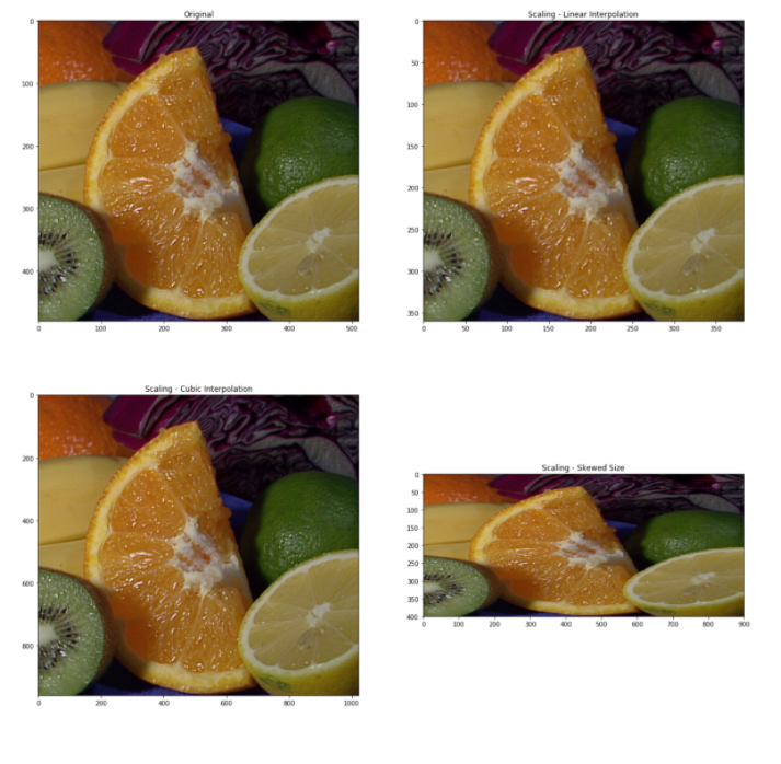
Re-sizing is one of the easiest tasks in OpenCV. It provides a resize() function which takes parameters such as image, output size image, interpolation, x scale, and y scale. Check the below code for complete implementation.
image = cv2.imread('/kaggle/input/opencv-samples-images/data/fruits.jpg')
image = cv2.cvtColor(image, cv2.COLOR_BGR2RGB)
plt.figure(figsize=(20, 20))
plt.subplot(2, 2, 1)
plt.title("Original")
plt.imshow(image)
image_scaled = cv2.resize(image, None, fx=0.75, fy=0.75)
plt.subplot(2, 2, 2)
plt.title("Scaling - Linear Interpolation")
plt.imshow(image_scaled)
img_scaled = cv2.resize(image, None, fx=2, fy=2, interpolation = cv2.INTER_CUBIC)
plt.subplot(2, 2, 3)
plt.title("Scaling - Cubic Interpolation")
plt.imshow(img_scaled)
img_scaled = cv2.resize(image, (900, 400), interpolation = cv2.INTER_AREA)
plt.subplot(2, 2, 4)
plt.title("Scaling - Skewed Size")
plt.imshow(img_scaled)
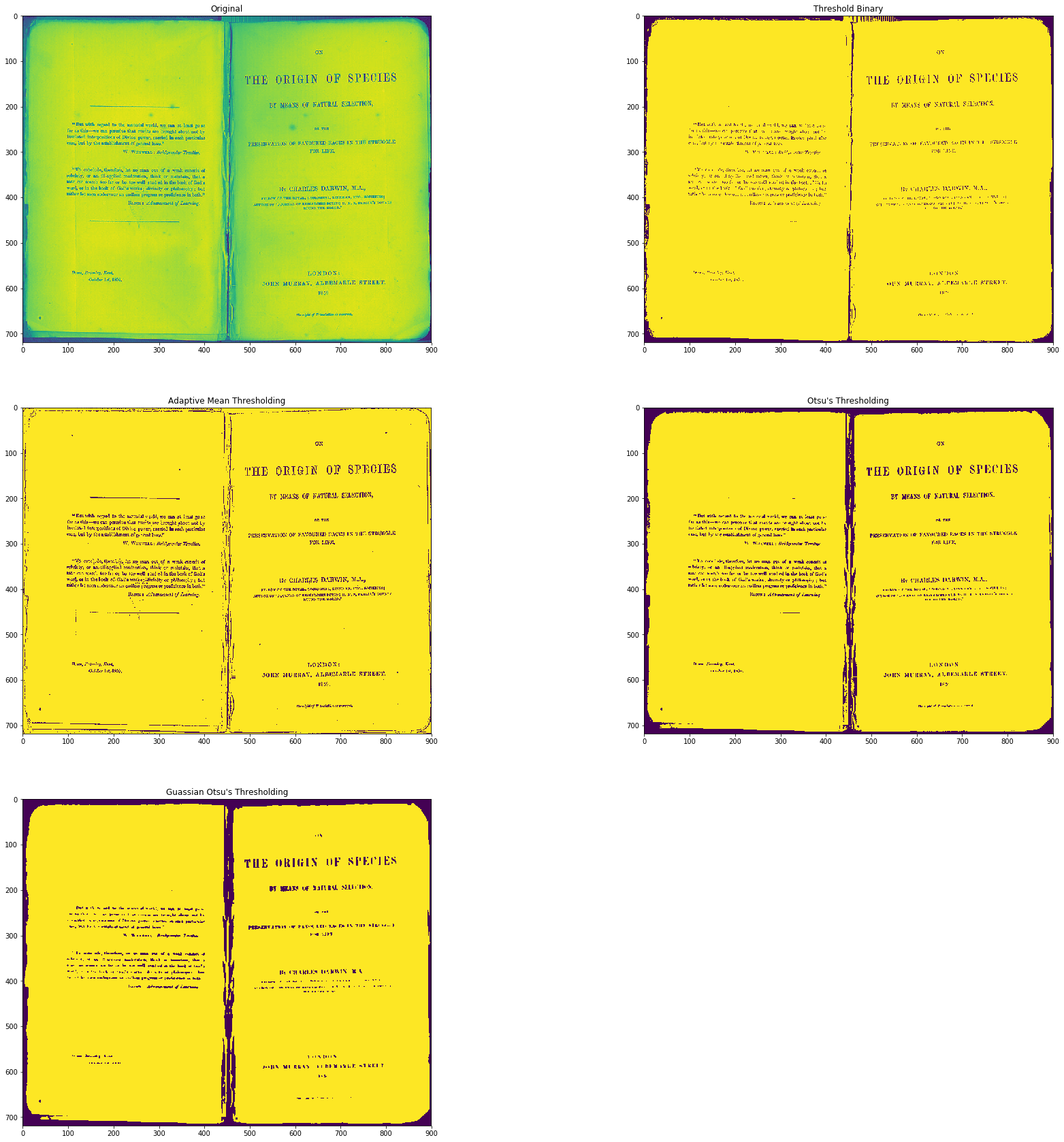
Check the below code for complete implementation. For more information, check this link.
# Load our new image
image = cv2.imread('Origin_of_Species.jpg', 0)
plt.figure(figsize=(30, 30))
plt.subplot(3, 2, 1)
plt.title("Original")
plt.imshow(image)
ret,thresh1 = cv2.threshold(image, 127, 255, cv2.THRESH_BINARY)
plt.subplot(3, 2, 2)
plt.title("Threshold Binary")
plt.imshow(thresh1)
image = cv2.GaussianBlur(image, (3, 3), 0)
thresh = cv2.adaptiveThreshold(image, 255, cv2.ADAPTIVE_THRESH_MEAN_C, cv2.THRESH_BINARY, 3, 5)
plt.subplot(3, 2, 3)
plt.title("Adaptive Mean Thresholding")
plt.imshow(thresh)
_, th2 = cv2.threshold(image, 0, 255, cv2.THRESH_BINARY + cv2.THRESH_OTSU)
plt.subplot(3, 2, 4)
plt.title("Otsu's Thresholding")
plt.imshow(th2)
plt.subplot(3, 2, 5)
blur = cv2.GaussianBlur(image, (5,5), 0)
_, th3 = cv2.threshold(blur, 0, 255, cv2.THRESH_BINARY + cv2.THRESH_OTSU)
plt.title("Guassian Otsu's Thresholding")
plt.imshow(th3)
plt.show()
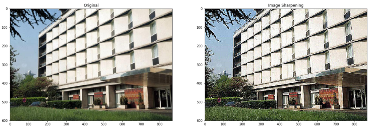
Check the below code for sharpening an image using OpenCV. For more information check this link
image = cv2.imread('building.jpg')
image = cv2.cvtColor(image, cv2.COLOR_BGR2RGB)
plt.figure(figsize=(20, 20))
plt.subplot(1, 2, 1)
plt.title("Original")
plt.imshow(image)
kernel_sharpening = np.array([[-1,-1,-1],
 [-1,9,-1],
 [-1,-1,-1]])
sharpened = cv2.filter2D(image, -1, kernel_sharpening)
plt.subplot(1, 2, 2)
plt.title("Image Sharpening")
plt.imshow(sharpened)
plt.show()
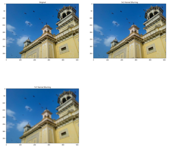
Check the below code for blurring an image using OpenCV. For more information check this link
image = cv2.imread('home.jpg')
image = cv2.cvtColor(image, cv2.COLOR_BGR2RGB)
plt.figure(figsize=(20, 20))
plt.subplot(2, 2, 1)
plt.title("Original")
plt.imshow(image)
kernel_3x3 = np.ones((3, 3), np.float32) / 9
blurred = cv2.filter2D(image, -1, kernel_3x3)
plt.subplot(2, 2, 2)
plt.title("3x3 Kernel Blurring")
plt.imshow(blurred)
kernel_7x7 = np.ones((7, 7), np.float32) / 49
blurred2 = cv2.filter2D(image, -1, kernel_7x7)
plt.subplot(2, 2, 3)
plt.title("7x7 Kernel Blurring")
plt.imshow(blurred2)
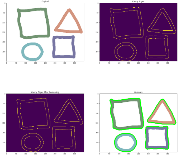
Image Contours – It is a way to identify the structural outlines of an object in an image. It is helpful to identify the shape of an object. OpenCV provides a findContours function in which you need to pass canny edges as a parameter. Check the below code for complete implementation. For more information, check this link.
# Load the data
image = cv2.imread('pic.png')
image = cv2.cvtColor(image, cv2.COLOR_BGR2RGB)
plt.figure(figsize=(20, 20))
plt.subplot(2, 2, 1)
plt.title("Original")
plt.imshow(image)
# Grayscale
gray = cv2.cvtColor(image,cv2.COLOR_BGR2GRAY)
# Canny edges
edged = cv2.Canny(gray, 30, 200)
plt.subplot(2, 2, 2)
plt.title("Canny Edges")
plt.imshow(edged)
# Finding Contours
contour, hier = cv2.findContours(edged, cv2.RETR_EXTERNAL, cv2.CHAIN_APPROX_NONE)
plt.subplot(2, 2, 3)
plt.imshow(edged)
print("Count of Contours = " + str(len(contour)))
# All contours
cv2.drawContours(image, contours, -1, (0,255,0), 3)
plt.subplot(2, 2, 4)
plt.title("Contours")
plt.imshow(image)
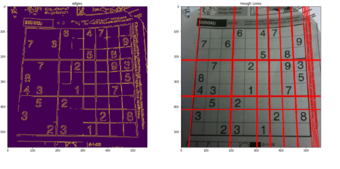
Lines can be detected in an image using Hough lines. OpenCV provides an HouhLines function in which you have to pass the threshold value. The threshold is the minimum vote for it to be considered a line. For a detailed overview, check the below code for complete implementation For line detection using Hough lines in OpenCV. For more information, check this link.
# Load the image
image = cv2.imread('sudoku.png')
image = cv2.cvtColor(image, cv2.COLOR_BGR2RGB)
plt.figure(figsize=(20, 20))
# Grayscale
gray = cv2.cvtColor(image, cv2.COLOR_BGR2GRAY)
# Canny Edges
edges = cv2.Canny(gray, 100, 170, apertureSize = 3)
plt.subplot(2, 2, 1)
plt.title("edges")
plt.imshow(edges)
# Run HoughLines Fucntion
lines = cv2.HoughLines(edges, 1, np.pi/180, 200)
# Run for loop through each line
for line in lines:
 rho, theta = line[0]
 a = np.cos(theta)
 b = np.sin(theta)
 x0 = a * rho
 y0 = b * rho
 x_1 = int(x0 + 1000 * (-b))
 y_1 = int(y0 + 1000 * (a))
 x_2 = int(x0 - 1000 * (-b))
 y_2 = int(y0 - 1000 * (a))
 cv2.line(image, (x_1, y_1), (x_2, y_2), (255, 0, 0), 2)
# Show Final output
plt.subplot(2, 2, 2)
plt.imshow(image)
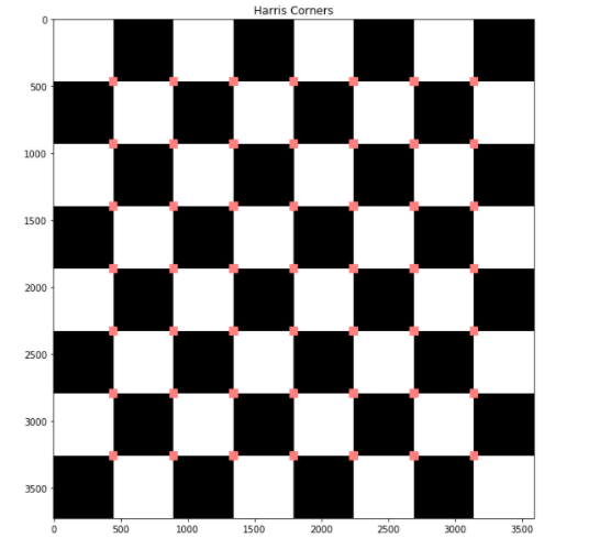
To find the corners of an image, use the cornerHarris function from OpenCV. For a detailed overview, check the below code for complete implementation to find corners using OpenCV. For more information, check this link.
# Load image
image = cv2.imread('chessboard.png')
# Grayscaling
image = cv2.cvtColor(image, cv2.COLOR_BGR2RGB)
plt.figure(figsize=(10, 10))
gray = cv2.cvtColor(image, cv2.COLOR_BGR2GRAY)
# CornerHarris function want input to be float
gray = np.float32(gray)
h_corners = cv2.cornerHarris(gray, 3, 3, 0.05)
kernel = np.ones((7,7),np.uint8)
h_corners = cv2.dilate(harris_corners, kernel, iterations = 10)
image[h_corners > 0.024 * h_corners.max() ] = [256, 128, 128]
plt.subplot(1, 1, 1)
# Final Output
plt.imshow(image)
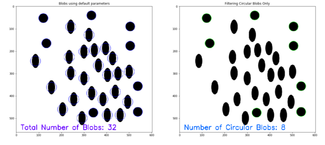
To Count Circles and Ellipse in an image, use the SimpleBlobDetector function from OpenCV. For a detailed overview, check the below code for complete implementation To Count Circles and Ellipse in an image using OpenCV. For more information, check this link.
# Load image
image = cv2.imread('blobs.jpg')
image = cv2.cvtColor(image, cv2.COLOR_BGR2RGB)
plt.figure(figsize=(20, 20))
detector = cv2.SimpleBlobDetector_create()
# Detect blobs
points = detector.detect(image)

blank = np.zeros((1,1))
blobs = cv2.drawKeypoints(image, points, blank, (0,0,255),
 cv2.DRAW_MATCHES_FLAGS_DRAW_RICH_KEYPOINTS)
number_of_blobs = len(keypoints)
text = "Total Blobs: " + str(len(keypoints))
cv2.putText(blobs, text, (20, 550), cv2.FONT_HERSHEY_SIMPLEX, 1, (100, 0, 255), 2)

plt.subplot(2, 2, 1)

plt.imshow(blobs)
# Filtering parameters
# Initialize parameter settiing using cv2.SimpleBlobDetector
params = cv2.SimpleBlobDetector_Params()
# Area filtering parameters
params.filterByArea = True
params.minArea = 100
# Circularity filtering parameters
params.filterByCircularity = True
params.minCircularity = 0.9
# Convexity filtering parameters
params.filterByConvexity = False
params.minConvexity = 0.2
# inertia filtering parameters
params.filterByInertia = True
params.minInertiaRatio = 0.01
# detector with the parameters
detector = cv2.SimpleBlobDetector_create(params)
# Detect blobs
keypoints = detector.detect(image)
# Draw blobs on our image as red circles
blank = np.zeros((1,1))
blobs = cv2.drawKeypoints(image, keypoints, blank, (0,255,0),
 cv2.DRAW_MATCHES_FLAGS_DRAW_RICH_KEYPOINTS)
number_of_blobs = len(keypoints)
text = "No. Circular Blobs: " + str(len(keypoints))
cv2.putText(blobs, text, (20, 550), cv2.FONT_HERSHEY_SIMPLEX, 1, (0, 100, 255), 2)
# Show blobs
plt.subplot(2, 2, 2)
plt.title("Filtering Circular Blobs Only")
plt.imshow(blobs)
So in this article, we had a detailed discussion on Image Processing Using OpenCV. Hope you learn something from this blog and it will help you in the future. Thanks for reading and your patience. Good luck!
You can check my articles here: Articles
Email id: [email protected]
Connect with me on LinkedIn: LinkedIn
The media shown in this article on Image Processing using OpenCV are not owned by Analytics Vidhya and is used at the Author’s discretion.
GPT-4 vs. Llama 3.1 – Which Model is Better?
Llama-3.1-Storm-8B: The 8B LLM Powerhouse Surpa...
A Comprehensive Guide to Building Agentic RAG S...
Top 10 Machine Learning Algorithms in 2026
45 Questions to Test a Data Scientist on Basics...
90+ Python Interview Questions and Answers (202...
8 Easy Ways to Access ChatGPT for Free
Prompt Engineering: Definition, Examples, Tips ...
What is LangChain?
What is Retrieval-Augmented Generation (RAG)?
Edit
Resend OTP
Resend OTP in 45s