Decision Tree Machine Learning Algorithm Using Python

5 min read

This article was published as a part of the Data Science Blogathon.

Introduction

In this article, we are going to learn about Decision Tree Machine Learning algorithm. We will build a Machine learning model using a decision tree algorithm and we use a news dataset for this. Nowadays fake news spread is like wildfire and this is a big issue. This dataset is a labelled dataset that contains labels as REAL or FAKE. It has title and text as independent features and label is a dependent feature.

When we provide the title and text inside news, our model is going to predict whether the news is REAL or FAKE.

Decision Tree Algorithm

Decision Tree is a supervised machine learning algorithm where all the decisions were made based on some conditions. The decision tree has a root node and leaf nodes extended from the root node. These nodes were decided based on some parameters like Gini index, entropy, information gain.

To know more about the decision tree algorithms, read my article.

In this article, I have explained the decision tree, and also I have taken one problem statement and have shown how to build a decision tree using Information gain, and all. Please have a look at it.

Link for the article:

Decision Tree Machine Learning Algorithm

Source: https://cdn.educba.com/academy/wp-content/uploads/2019/11/Decision-Tree-in-Machine-Learning.png

Working with Dataset

Before creating and training our model, first, we have to preprocess our dataset.

Let us start by Importing some important basic libraries.

import pandas as pd
import numpy as np
import seaborn as sns
import matplotlib.pyplot as plt
import warnings
warnings.simplefilter("ignore")

To just ignore warnings that we come across during model creation, just import warnings and set it to ignore.

Seaborn and Matplotlib are two famous libraries that are used for visualizations.

Coming to the dataset, here is the link. Click on it to download.

https://bit.ly/3FxCSC4

Now import it from your local desktop. Paste the path to the news file in the read_csv. Use pandas for it.

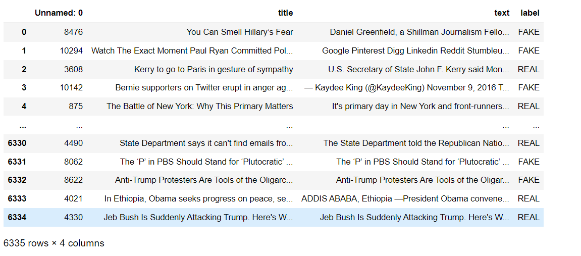
Now view it. To view the data frame that you have created simply enter the name of the data frame and run. Instead of showing all the rows, it will give the first five rows and the last five rows.

import pandas as pd
df = pd.read_csv('news.csv')
print(df)

View the info of the data frame.

df.info()

RangeIndex: 6335 entries, 0 to 6334
Data columns (total 4 columns):
 # Column Non-Null Count Dtype 
--- ------ -------------- ----- 
 0 Unnamed: 0 6335 non-null int64 
 1 title 6335 non-null object
 2 text 6335 non-null object
 3 label 6335 non-null object
dtypes: int64(1), object(3)
memory usage: 198.1+ KB

Check for null values. Use the is null method for it.

df.isnull().sum()

Unnamed: 0 0
title 0
text 0
label 0
dtype: int64

We can see that all values are 0. It shows that there are no null values in the dataset. So we can move further without changing anything in the dataset.

View the shape. This shaping method gives the number of rows and the number of columns in it.

print("There are {} rows and {} columns.".format(df.shape[0],df.shape[1]))

There are 6335 rows and 4 columns.

View the statistical description of the data frame. The statistical description shows details like count (non-null values in the column), mean, standard deviation, minimum value, maximum values, and finally percentiles of the values in that column. In our data frame, we have only one numerical column so it will give a description for only one column. But we don’t need this column for building our model.

df.describe()

	Unnamed: 0
count	6335.000000
mean	5280.415627
std	3038.503953
min	2.000000
25%	2674.500000
50%	5271.000000
75%	7901.000000
max	10557.000000

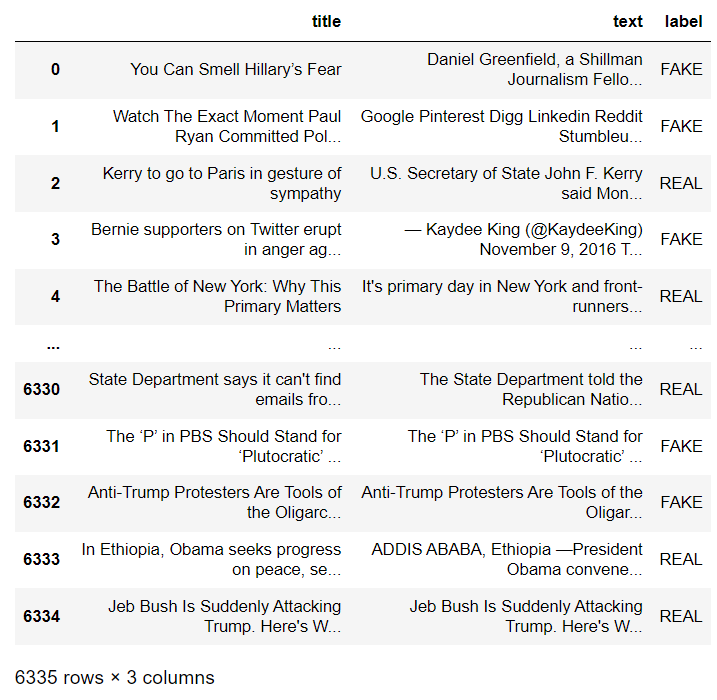
Drop this unnamed column using the drop method.

#Let's drop unimportant columns
df=df.drop(['Unnamed: 0'],axis=1)

Now view the final updated data frame.

df

Let us see how much Real news and how much Fake news was there in the dataset. The value counts method actually returns the count of a particular variable in a given feature.

df['label'].value_counts()

REAL 3171
FAKE 3164
Name: label, dtype: int64

There are 3171 Real news and 3164 Fake news. OMG!! probability is almost 0.5 for the news being fake so, be aware of them.

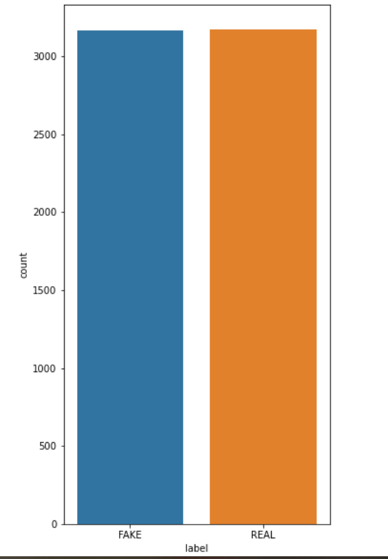
Visualizations

Visualize the count plot using the seaborn library.

plt.figure(figsize=(5,10));
sns.countplot(df['label']);

In the graph, we can see that both are almost similar.

Define x and y.

For creating a model, first, we have to define x and y in which x contains all independent features of the dataset and y contains a dependent feature that is labelled.

x = df.iloc[ : , :-1].values
y = df.iloc[ : , -1].values

Import CountVectorizer

As we are working with text data, we have to use a count vectorizer for it. It is actually used to transform our text into a vector on the basis of the frequency of each word which means how many times the word is repeated in the entire text.

It is available in the sci-kit learn library.

Fit_transform is used on the training dataset because it will scale our training data and learn the scaling parameters. With this, our model will learn the mean and variance of the features that are there in this training dataset. These parameters are used to work with test data.

from sklearn.feature_extraction.text import CountVectorizer
vect=CountVectorizer(stop_words="english",max_features=1000)

x1=vect.fit_transform(x[:,0]).todense()
x2=vect.fit_transform(x[:,1]).todense()
x_mat=np.hstack((x1,x2))

Let’s view the final matrix that was created.

x_mat

matrix([[0, 0, 0, ..., 0, 2, 0],
 [0, 0, 0, ..., 0, 0, 0],
 [0, 0, 0, ..., 0, 0, 0],
 ...,
 [0, 0, 0, ..., 0, 0, 0],
 [0, 0, 0, ..., 0, 0, 0],
 [0, 0, 0, ..., 0, 0, 0]], dtype=int64)

Split the data into train and test datasets

For this, you have to import train_test_split which is available in the sci-kit learn library.

from sklearn.model_selection import train_test_split
x_train,x_test,y_train,y_test= train_test_split(x_mat,y,random_state=1000)

Create Model

Import DecisionTreeClassifier and set criterion to entropy so that our model will build a decision tree taking entropy as criteria and assigning it to a variable called a model. So from now on whenever we need to use DecisionTreeClassifier(criterion=”entropy”), we just have to use the model.

Train the model

Train the model using the fit method and pass training datasets as arguments in it.

model.fit(x_train,y_train)

DecisionTreeClassifier(criterion=’entropy’)

It’s time to predict the results. Use predict method for it.

y_pred=model.predict(x_test)

View the predicted results.

y_pred

array([‘FAKE’, ‘REAL’, ‘REAL’, …, ‘REAL’, ‘REAL’, ‘REAL’], dtype=object)

Find Accuracy of the Model

Now we will see the accuracy and confusion matrix for the model that we built.

For that import accuracy_score and confusion_matrix from the sci-kit learn library.

from sklearn.metrics import accuracy_score,confusion_matrix

accuracy=accuracy_score(y_pred,y_test)*100
print("Accuracy of the model is {:.2f}".format(accuracy))

The accuracy of the model is 79.61

confusion_matrix(y_pred,y_test)

array([[632, 174],
 [149, 629]], dtype=int64)

We can see that accuracy of our model is 79.61 per cent.

Conclusion

–> In this article, we have seen how to build a decision tree algorithm.

–> For this, we have used a news dataset that has labelled as Real or Fake.

–> Finally, we got an accuracy score of 79.61%.

Hope you guys found it useful.

Connect with me on Linkedin: https://www.linkedin.com/in/amrutha-k-6335231a6vl/

Read the latest article on our website.

Thanks!!

The media shown in this article is not owned by Analytics Vidhya and are used at the Author’s discretion.

Login to continue reading and enjoy expert-curated content.

Free Courses

Become an Author

Share insights, grow your voice, and inspire the data community.

• Reach a Global Audience
• Share Your Expertise with the World
• Build Your Brand & Audience

• Join a Thriving AI Community
• Level Up Your AI Game
• Expand Your Influence in Genrative AI

👁 imag