Local Search Algorithms in Artificial Intelligence are optimization techniques that improve a solution by repeatedly moving to a better neighbouring state. Instead of exploring every possible path, they focus on finding efficient and practical solutions for complex problems.
Improve solutions through neighbouring states
Useful for optimization and decision-making problems
Commonly used in scheduling, routing, and machine learning tasks
Basic Terminologies
State: A possible solution to the problem
Current State: The solution currently being evaluated
Neighbour State: A solution formed by making small changes to the current state
Objective Function: A function used to measure the quality of a solution
Local Optimum: The best solution among nearby states
Global Optimum: The best possible solution in the entire search space
Working
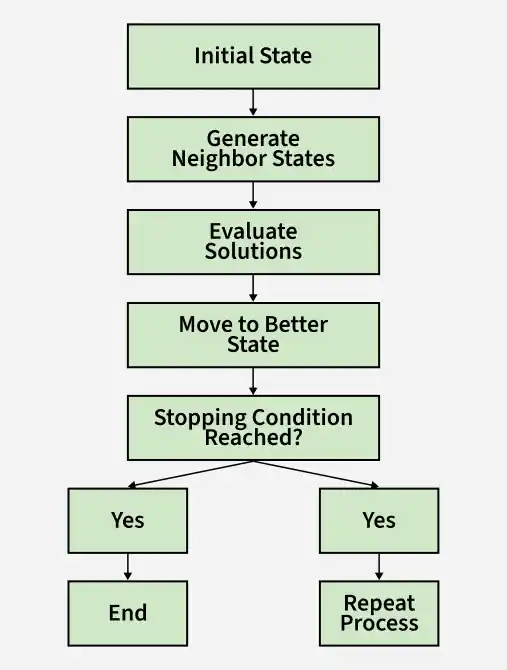
1. Pick a starting point: Start with a possible solution which is often random but sometimes based on rule.
2. Find the Neighbours:
Neighbours are similar solutions we can get by making small, simple changes to the current one.
For example, in a puzzle, swapping two pieces creates a neighbour.
3. Compare: Look around at all neighbors to see if any are better.
4. Move: If a better neighbor exists, move to it, making it our new “current” solution.
5. Repeat: Keep searching from the new point, following the same steps.
6. Stop: When none of the neighbors are better or after enough tries.
Hill-Climbing search algorithm is a simple local search algorithm that continuously moves toward a better neighboring solution until no improvement is possible.
Process:
Start: Begin with an initial solution.
Evaluate: Assess the neighboring solutions.
Move: Transition to the neighbor with the highest objective function value if it improves the current solution.
Repeat: Continue this process until no better neighboring solution exists.
Pros:
Easy to implement.
Works well in small or smooth search spaces.
Cons:
May get stuck in local optima.
Limited exploration of the search space.
Output: Found maximum at x = 3.02, value = 5.00
2. Simulated Annealing
Simulated Annealing is a local search algorithm inspired by the heating and cooling process in metallurgy. It occasionally accepts worse solutions to escape local optima, with the acceptance probability decreasing over time.
Process:
Start: Begin with an initial solution and an initial temperature.
Move: Transition to a neighboring solution with a certain probability.
Cooling Schedule: Gradually reduce the temperature over time.
Probability Function: Accept worse solutions with decreasing probability as temperature lowers.
Pros:
Helps escape local optima due to probabilistic acceptance of worse solutions.
Explores the search space more effectively.
Cons:
Requires careful parameter tuning.
Computationally expensive due to repeated evaluations.
Output: Best found x = 3.02, value = 4.96
3. Genetic Algorithms
Genetic Algorithms (GAs) are inspired by the process of natural selection and evolution. They work with a population of solutions and evolve them over time using genetic operators like selection, crossover and mutation.
Process:
Initialize: Start with a population of random solutions.
Evaluate: Assess the fitness of each solution.
Select: Choose the best solutions for reproduction based on their fitness.
Crossover: Combine pairs of solutions to produce new offspring.
Mutate: Apply random changes to offspring to maintain diversity.
Replace: Form a new population by selecting which solutions to keep.
Pros:
Can explore a broad solution space and find high-quality solutions.
Suitable for complex problems with large search spaces.
Cons:
Can be computationally expensive
Requires tuning of various parameters like population size and mutation rate.
Output: Best found x = 3.00, value = 5.00
4. Tabu Search
Tabu Search enhances local search by using a memory structure called the tabu list to avoid revisiting previously explored solutions. This helps to prevent cycling back to local optima and encourages exploration of new areas.
Process:
Start: Begin with an initial solution and initialize the tabu list.
Move: Transition to a neighboring solution while considering the tabu list.
Update: Add the current solution to the tabu list and potentially remove older entries.
Aspiration Criteria: Allow moves that lead to better solutions even if they are in the tabu list.
Pros:
Reduces the chance of getting stuck in local optima.
Effective in exploring large and complex search spaces.
Cons:
Requires careful management of the tabu list and aspiration criteria.
Computational complexity can be high.
Output: Best found x = 3.02, value = 5.00
Comparison of Local Search Algorithms
Feature
Hill-Climbing
Simulated Annealing
Genetic Algorithm
Tabu Search
Search Style
Local search
Probabilistic search
Population-based search
Memory-based search
Moves to Worse Solutions
No
Yes
Yes
Rarely
Avoids Local Optima
No
Yes
Yes
Yes
Speed
Fast
Moderate
Slower
Moderate
Best Use Case
Small problems
Problems with many local optima
Complex optimization problems
Problems with repeated states
Applications
Scheduling: Creating timetables for schools, jobs, or exams while avoiding conflicts
Routing: Finding efficient paths for delivery and travel problems such as the Traveling Salesperson Problem
Resource Allocation: Assigning limited resources like machines, rooms, or staff efficiently
Games and AI: Making fast decisions and strategic moves in complex games
Machine Learning: Tuning model parameters to improve performance
Advantages
Require less memory compared to exhaustive search methods
Work efficiently for large and complex search spaces
