 |
VOOZH | about |
|
VOOZH | about |
Time series forecasting plays a major role in data analysis, with applications ranging from anticipating stock market trends to forecasting weather patterns. In this article, we'll dive into the field of time series forecasting using PyTorch and LSTM (Long Short-Term Memory) neural networks. We'll uncover the critical preprocessing procedures that underpin the accuracy of our forecasts along the way.
Time series data is essentially a set of observations taken at regular periods of time. Time series forecasting attempts to estimate future values based on patterns and trends detected in historical data. Moving averages and traditional approaches like ARIMA have trouble capturing long-term dependencies in the data. LSTM is a type of recurrent neural network, that excels at capturing dependencies through time and able to intricate patterns.
Here, we have used Yahoo Finance to get the share market dataset.
To install the Yahoo Finance, we can use the following command
!pip install yfinanceThis step involves importing various libraries essential for data processing, visualization, machine learning, and deep learning tasks.
Download the historical stock price data for Apple Inc. (AAPL) from Yahoo Finance. Inspect the data using df.head() and df.info() to understand its structure and contents.
Output:
[*********************100%***********************] 1 of 1 completed

 Open High Low Close Volume
Date
1990-01-02 0.261498 0.263253 0.245703 0.247458 183198400
1990-01-03 0.263253 0.266764 0.263253 0.266764 207995200
1990-01-04 0.264132 0.272029 0.261498 0.268519 221513600
1990-01-05 0.265009 0.268519 0.259744 0.265009 123312000
1990-01-08 0.266764 0.266764 0.259744 0.263253 101572800
<class 'pandas.core.frame.DataFrame'>
DatetimeIndex: 8940 entries, 1990-01-02 to 2025-07-01
Data columns (total 5 columns):
 # Column Non-Null Count Dtype
--- ------ -------------- -----
 0 Open 8940 non-null float64
 1 High 8940 non-null float64
 2 Low 8940 non-null float64
 3 Close 8940 non-null float64
 4 Volume 8940 non-null int64
dtypes: float64(4), int64(1)
memory usage: 419.1 KB
None
Define a function to plot the data using line plots for each column in the DataFrame. This helps visualize trends and patterns in the data.
Output:
In this step, we split the data into training and testing sets, and normalize the values using MinMaxScaler. This preprocessing is essential for preparing the data for machine learning models.
math.ceil: Used to calculate the number of training data points (80% of the total data).train_data and test_data: Split the DataFrame into training and testing sets.MinMaxScaler: Scales the data to a range of [0, 1]. This normalization helps the neural network to converge faster.Output:
7152
(7152, 1) (1788, 1)
(7152, 1)
(1788, 1)
[[0.00367675]
 [0.00371602]
 [0.00373567]
 [0.00375531]
 [0.00379458]]
[[0.04682367]
 [0.04632846]
 [0.04759275]
 [0.04737147]
 [0.04782451]]
We structure the data into sequences for the LSTM model. Each sequence contains a specified number of time steps. We then convert the data into PyTorch tensors, which are necessary for input into the PyTorch model.
sequence_length: The number of time steps the model looks back to make a prediction.X_train and y_train: Arrays to hold the input sequences and their corresponding labels for training.X_test and y_test: Arrays for testing data.torch.tensor: Converts the numpy arrays into PyTorch tensors.Output:
torch.Size([7102, 50, 1]) torch.Size([7102, 1])
torch.Size([1758, 30, 1]) torch.Size([1758, 1])
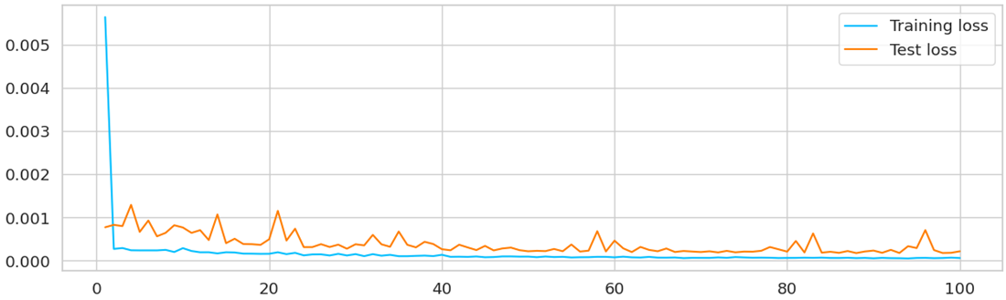
Define an LSTM model for time series forecasting. The model includes an LSTM layer followed by a fully connected layer. Train the model using the training data and evaluate it on the test data.
Output:
cuda
Epoch [10/100] - Training Loss: 0.0003, Test Loss: 0.0008
Epoch [20/100] - Training Loss: 0.0002, Test Loss: 0.0005
Epoch [30/100] - Training Loss: 0.0002, Test Loss: 0.0004
Epoch [40/100] - Training Loss: 0.0001, Test Loss: 0.0003
Epoch [50/100] - Training Loss: 0.0001, Test Loss: 0.0002
Epoch [60/100] - Training Loss: 0.0001, Test Loss: 0.0005
Epoch [70/100] - Training Loss: 0.0001, Test Loss: 0.0002
Epoch [80/100] - Training Loss: 0.0001, Test Loss: 0.0002
Epoch [90/100] - Training Loss: 0.0001, Test Loss: 0.0002
Epoch [100/100] - Training Loss: 0.0001, Test Loss: 0.0002
Output:
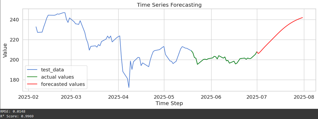
Use the trained model to forecast future values. Evaluate the model's performance using metrics like RMSE and R² score.
Output:
By plotting the test data, actual values and model's forecasting data. We got a clear idea of how well the forecasted values are aligning with the actual time series.
The intriguing field of time series forecasting using PyTorch and LSTM neural networks has been thoroughly examined in this paper. In order to collect historical stock market data using Yahoo Finance module, we imported the yfinance library and started the preprocessing step. Then we applied crucial actions like data loading, train-test splitting, and data scaling to make sure our model could accurately learn from the data and make predictions.
For more accurate forecasts, additional adjustments, hyperparameter tuning, and optimization are frequently needed. To improve predicting capabilities, ensemble methods and other cutting-edge methodologies can be investigated.
We have barely begun to explore the enormous field of time series forecasting in this essay. There is a ton more to learn, from managing multi-variate time series to resolving practical problems in novel ways. With this knowledge in hand, you're prepared to use PyTorch and LSTM neural networks to go out on your own time series forecasting adventures.
Enjoy your forecasting!
Notebook: click here.