 |
VOOZH | about |
|
VOOZH | about |
Recurrent Neural Networks (RNNs) are a class of neural networks designed to process sequential data by retaining information from previous steps. They are especially effective for tasks where context and order matter.
Imagine reading a sentence and you try to predict the next word, you don’t rely only on the current word but also remember the words that came before. RNNs work similarly by “remembering” past information i.e it considers all the earlier words to choose the most likely next word.
This memory of previous steps helps the network understand context and make better predictions.
There are mainly two components of RNNs that we will discuss.
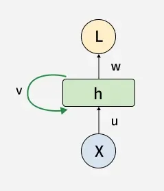
The fundamental processing unit in RNN is a Recurrent Unit. They hold a hidden state that maintains information about previous inputs in a sequence. Recurrent units can "remember" information from prior steps by feeding back their hidden state, allowing them to capture dependencies across time.
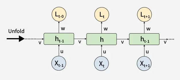
RNN unfolding or unrolling is the process of expanding the recurrent structure over time steps. During unfolding each step of the sequence is represented as a separate layer in a series illustrating how information flows across each time step.
This unrolling enables backpropagation through time (BPTT) a learning process where errors are propagated across time steps to adjust the network’s weights enhancing the RNN’s ability to learn dependencies within sequential data.
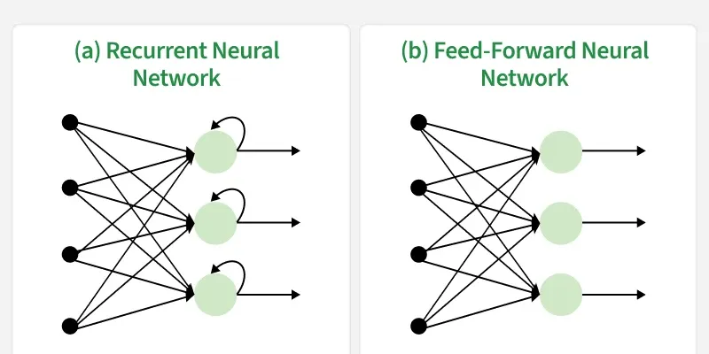
RNNs share similarities in input and output structures with other deep learning architectures but differ significantly in how information flows from input to output. Unlike traditional deep neural networks where each dense layer has distinct weight matrices. RNNs use shared weights across time steps, allowing them to remember information over sequences.
In RNNs the hidden state is calculated for every input to retain sequential dependencies. The computations follow these core formulas:
1. Hidden State Calculation:
Here:
2. Output Calculation:
The output is calculated by applying an activation function to the weighted hidden state where and represent weights and bias.
3. Overall Function:
This function defines the entire RNN operation where the state matrix holds each element representing the network's state at each time step .
At each time step RNNs process units with a fixed activation function. These units have an internal hidden state that acts as memory that retains information from previous time steps. This memory allows the network to store past knowledge and adapt based on new inputs.
The current hidden state depends on the previous state and the current input and is calculated using the following relations:
1. State Update:
where:
2. Activation Function Application:
Here, is the weight matrix for the recurrent neuron and is the weight matrix for the input neuron.
3. Output Calculation:
where is the output and is the weight at the output layer.
These parameters are updated using backpropagation. However, since RNN works on sequential data here we use an updated backpropagation which is known as backpropagation through time.
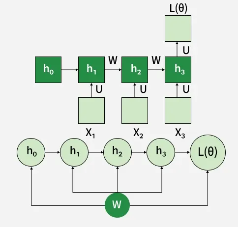
Since RNNs process sequential data, Backpropagation Through Time (BPTT) is used to update the network's parameters. The loss function L(θ) depends on the final hidden state and each hidden state relies on preceding ones forming a sequential dependency chain:
.
In BPTT, gradients are backpropagated through each time step. This is essential for updating network parameters based on temporal dependencies.
1. Simplified Gradient Calculation:
2. Handling Dependencies in Layers: Each hidden state is updated based on its dependencies:
The gradient is then calculated for each state, considering dependencies from previous hidden states.
3. Gradient Calculation with Explicit and Implicit Parts: The gradient is broken down into explicit and implicit parts summing up the indirect paths from each hidden state to the weights.
4. Final Gradient Expression: The final derivative of the loss function with respect to the weight matrix W is computed:
This iterative process is the essence of backpropagation through time.
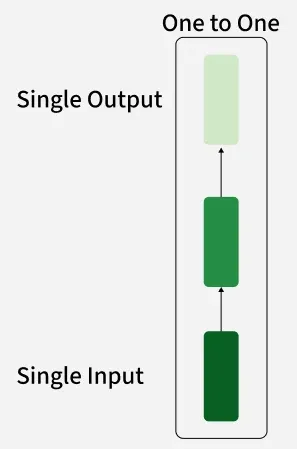
There are four types of RNNs based on the number of inputs and outputs in the network:
This is the simplest type of neural network architecture where there is a single input and a single output. It is used for straightforward classification tasks such as binary classification where no sequential data is involved.
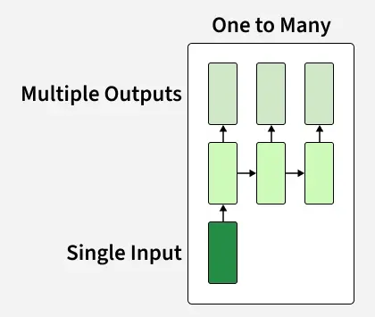
In a One-to-Many RNN the network processes a single input to produce multiple outputs over time. This is useful in tasks where one input triggers a sequence of predictions (outputs). For example in image captioning a single image can be used as input to generate a sequence of words as a caption.
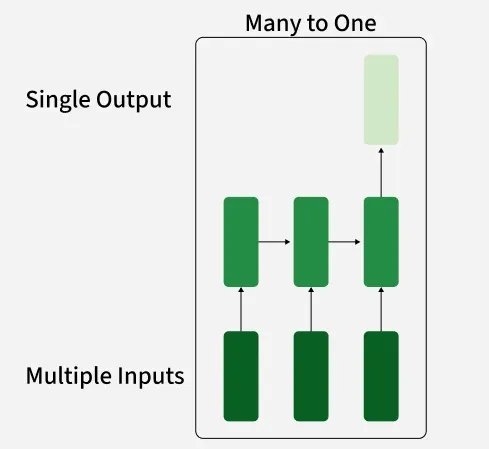
The Many-to-One RNN receives a sequence of inputs and generates a single output. This type is useful when the overall context of the input sequence is needed to make one prediction. In sentiment analysis the model receives a sequence of words (like a sentence) and produces a single output like positive, negative or neutral.
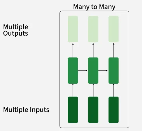
The Many-to-Many RNN type processes a sequence of inputs and generates a sequence of outputs. In language translation task a sequence of words in one language is given as input and a corresponding sequence in another language is generated as output.
There are several variations of RNNs, each designed to address specific challenges or optimize for certain tasks:
This simplest form of RNN consists of a single hidden layer where weights are shared across time steps. Vanilla RNNs are suitable for learning short-term dependencies but are limited by the vanishing gradient problem, which hampers long-sequence learning.
Bidirectional RNNs process inputs in both forward and backward directions, capturing both past and future context for each time step. This architecture is ideal for tasks where the entire sequence is available, such as named entity recognition and question answering.
Long Short-Term Memory Networks (LSTMs) introduce a memory mechanism to overcome the vanishing gradient problem. Each LSTM cell has three gates:
Gated Recurrent Units (GRUs) simplify LSTMs by combining the input and forget gates into a single update gate and streamlining the output mechanism. This design is computationally efficient, often performing similarly to LSTMs and is useful in tasks where simplicity and faster training are beneficial.
In this section, we create a character-based text generator using Recurrent Neural Network (RNN) in TensorFlow and Keras. We'll implement an RNN that learns patterns from a text sequence to generate new text character-by-character.
We start by importing essential libraries for data handling and building the neural network.
We define the input text and identify unique characters in the text which we’ll encode for our model.
To train the RNN, we need sequences of fixed length (seq_length) and the character following each sequence as the label.
For training we convert X and y into one-hot encoded tensors.
We create a simple RNN model with a hidden layer of 50 units and a Dense output layer with softmax activation.
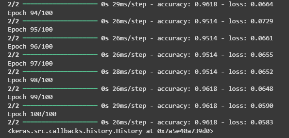
We compile the model using the categorical_crossentropy loss and train it for 100 epochs.
Output:
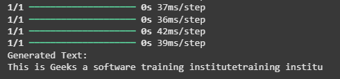
After training we use a starting sequence to generate new text character by character.
Output:
You can download source code from here.
While RNNs excel at handling sequential data they face two main training challenges i.e vanishing gradient and exploding gradient problem: