Linear Regression in Machine learning

Linear Regression is a fundamental supervised learning algorithm used to model the relationship between a dependent variable and one or more independent variables. It predicts continuous values by fitting a straight line that best represents the data.

• It assumes that there is a linear relationship between the input and output
• Uses a best‑fit line to make predictions
• Commonly used in forecasting, trend analysis, and predictive modelling

For example, suppose we want to predict a student’s exam score based on the number of hours studied. As study hours increase, exam scores generally increase as well. Here:

• Independent variable (input): Hours studied because it's the factor we control or observe.
• Dependent variable (output): Exam score because it depends on how many hours were studied.

Linear regression uses the independent variable to predict the dependent variable.

Best Fit Line

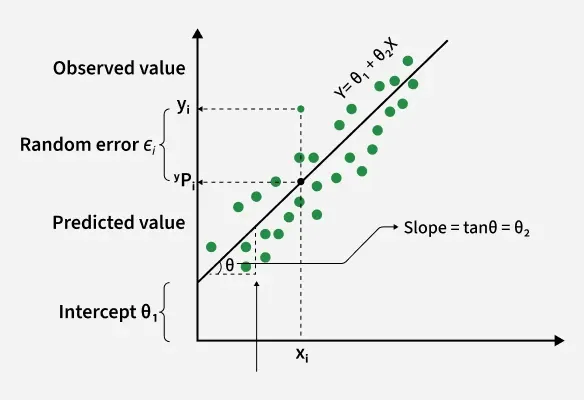
In linear regression, the best-fit line is the straight line that best represents the relationship between the independent variable (input) and the dependent variable (output). The goal is to minimize the difference between the actual data points and the predicted values generated by the model.

1. Goal of the Best-Fit Line

The goal of linear regression is to find a straight line that minimizes the error (the difference) between the observed data points and the predicted values. This line helps us predict the dependent variable for new, unseen data.

Here Y is called a dependent or target variable and X is called an independent variable also known as the predictor of Y.

• represents the intercept, which is the value of Y when X = 0
• represents the slope, which shows how much Y changes for a unit change in X

There are many types of functions or modules that can be used for regression. A linear function is the simplest type of function. Here, X may be a single feature or multiple features representing the problem.

2. Equation of the Best-Fit Line

For simple linear regression (with one independent variable), the best-fit line is represented by the equation

Where:

• y is the predicted value (dependent variable)
• x is the input (independent variable)
• m is the slope of the line (how much y changes when x changes)
• b is the intercept (the value of y when x = 0)

The best-fit line will be the one that optimizes the values of m (slope) and b (intercept) so that the predicted y values are as close as possible to the actual data points.

3. Minimizing the Error using the Least Squares Method

To determine the best-fit line, linear regression uses the Least Squares Method, which minimizes the difference between actual and predicted values. These differences are called residuals. These differences are called residuals.

The formula for residuals is:

Residual =

Where:

• is the actual observed value
• is the predicted value from the line for that

The least squares method minimizes the sum of the squared residuals:

This method ensures that the line best represents the data where the sum of the squared differences between the predicted values and actual values is as small as possible.

4. Interpretation of the Best-Fit Line

• Slope (m): The slope indicates how much the dependent variable changes for every one-unit increase in the independent variable. For example, if the slope is 5, then y increases by 5 units for every 1-unit increase in x.
• Intercept (b): The intercept represents the predicted value of y when x = 0. It’s the point where the line crosses the y-axis.

In linear regression some hypothesis are made to ensure reliability of the model's results.

Limitations:

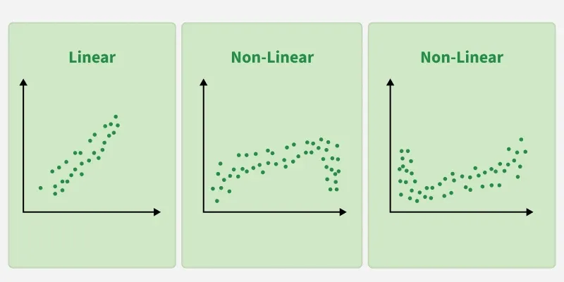
• Assumes Linearity: The method assumes the relationship between the variables is linear. If the relationship is non-linear, linear regression might not work well.
• Sensitivity to Outliers: Outliers can significantly affect the slope and intercept, skewing the best-fit line.

Hypothesis Function

In linear regression, the hypothesis function is the equation used to make predictions about the dependent variable based on the independent variables. It represents the relationship between the input features and the target output.

For a simple case with one independent variable, the hypothesis function is:

Where:

• or is the predicted value of the dependent variable (y).
• is the independent variable.
• is the intercept, representing the value of y when x is 0.
• is the slope, indicating how much y changes for each unit change in x.

For multiple linear regression (with more than one independent variable), the hypothesis function expands to:

Where:

• are the independent variables.
• is the intercept.
• are the coefficients, representing the influence of each respective independent variable on the predicted output.

Cost Function

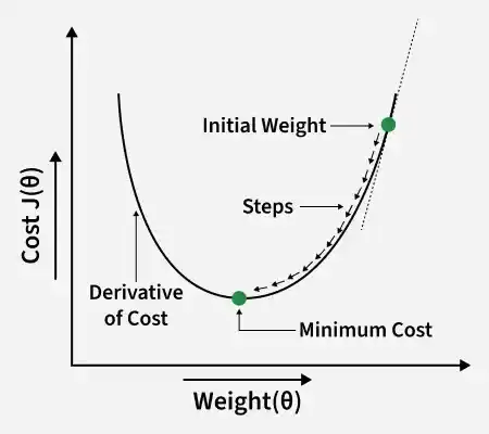
In Linear Regression, the cost function measures how far the predicted values are from the actual values (Y). It helps identify and reduce errors to find the best-fit line. The most common cost function used is Mean Squared Error (MSE), which calculates the average of squared differences between actual and predicted values.

Here:

• : It is used to minimize this cost, we use Gradient Descent, which iteratively updates θ₁ and θ₂​ until the MSE reaches its lowest value. This ensures the line fits the data as accurately as possible.

Gradient Descent

Gradient descent is an optimization technique used to train a linear regression model by minimizing the prediction error. It works by starting with random model parameters and repeatedly adjusting them to reduce the difference between predicted and actual values.

How it works:

• Start with random values for slope and intercept.
• Calculate the error between predicted and actual values.
• Find how much each parameter contributes to the error (gradient).
• Update the parameters in the direction that reduces the error.
• Repeat until the error is as small as possible.

This helps the model find the best-fit line for the data.

Types of Linear Regression

When there is only one independent feature it is known as Simple Linear Regression or Univariate Linear Regression and when there are more than one feature it is known as Multiple Linear Regression or Multivariate Regression.

1. Simple Linear Regression

Simple linear regression is used when we want to predict a target value (dependent variable) using only one input feature (independent variable). It assumes a straight-line relationship between the two.

Formula:

Where:

• is the predicted value
• is the input (independent variable)
• is the intercept (value of when x=0)
• is the slope or coefficient (how much changes with one unit of x)

Example: Predicting a person’s salary (y) based on their years of experience (x).

2. Multiple Linear Regression

Multiple linear regression involves more than one independent variable and one dependent variable. The equation for multiple linear regression is:

Where:

• is the predicted value
• are the independent variables
• are the coefficients (weights) corresponding to each predictor
• is the intercept

The goal is to find the best-fit line that predicts Y accurately for given inputs X.

Use Cases:

• Real Estate: Predict property prices using location, size and other factors.
• Finance: Forecast stock prices using interest rates and inflation data.
• Agriculture: Estimate crop yield from rainfall, temperature and soil quality.
• E-commerce: Analyze how price, promotions and seasons affect sales.

Assumptions of the Linear Regression

1. Linearity: The relationship between inputs (X) and the output (Y) is a straight line.

2. Independence of Errors: The errors in predictions should not affect each other.

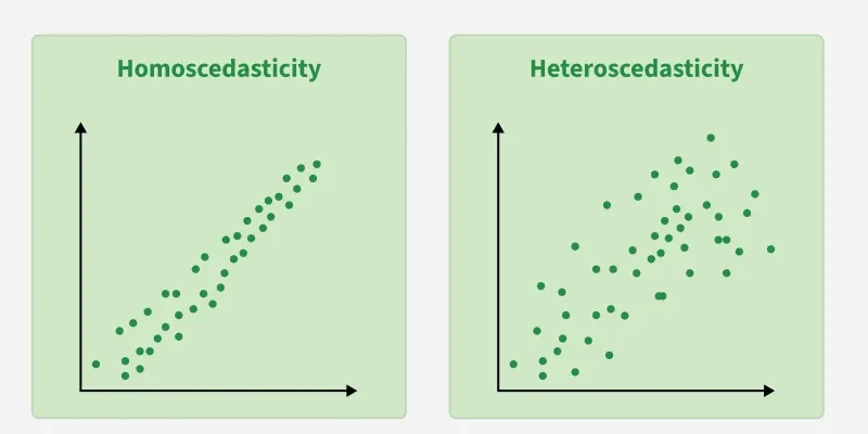
3. Constant Variance (Homoscedasticity): The errors should have equal spread across all values of the input. If the spread changes (like fans out or shrinks), it's called heteroscedasticity and it's a problem for the model.

4. Normality of Errors: The errors should follow a normal (bell-shaped) distribution.

5. No Multicollinearity (for multiple regression): Input variables shouldn’t be too closely related to each other.

6. No Autocorrelation: Errors shouldn't show repeating patterns, especially in time-based data.

7. Additivity: The total effect on Y is just the sum of effects from each X, no mixing or interaction between them.

To understand Multicollinearity in detail refer to this article: Multicollinearity.

Evaluation Metrics

A variety of evaluation measures can be used to determine the strength of any linear regression model. These assessment metrics often give an indication of how well the model is producing the observed outputs.

• Mean Squared Error (MSE): Measures the average squared difference between actual and predicted values to avoid cancellation of errors.
• Mean Absolute Error (MAE): Calculate the accuracy of a regression model. MAE measures the average absolute difference between the predicted values and actual values.
• Root Mean Squared Error (RMSE): Square root of the residuals variance is RMSE. It describes how well the observed data points match the expected values or the model's absolute fit to the data.
• R-Squared: Indicates how much variation the model explains. Its value is typically between 0 and 1, but it can be negative if the model performs worse than a simple baseline model (e.g., predicting the mean).
• Adjusted R-square: Measures the proportion of variance explained by the model while adjusting for the number of predictors and penalizing irrelevant features.

Regularization Techniques

• Lasso Regression: Regularizes a linear regression model, it adds a penalty term to the linear regression objective function to prevent overfitting.
• Ridge regression: Adds a regularization term to the standard linear objective to prevent overfitting by penalizing large coefficient in linear regression equation. It useful when the dataset has multicollinearity where predictor variables are highly correlated.
• Elastic Net Regression: Hybrid regularization technique that combines the power of both L1 and L2 regularization in linear regression objective.

Implementation

1. Import the necessary libraries

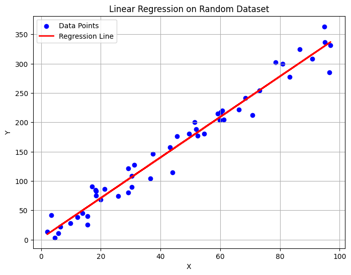
Importing NumPy for numerical operations, Matplotlib for visualization, and Scikit-learn for building the linear regression model.

2. Generating Random Dataset

Creating a sample input and output data for training the linear regression model.

3. Creating and Training Linear Regression Model

Initialize the model and train it using the generated dataset.

4. Predicting Y Values

Using the trained model to predict output values for the input data.

5. Visualizing the Regression Line

Plot the original data points along with the best-fit regression line.

Output:

6. Slope and Intercept

Print the learned slope and intercept values of the regression model.

Output:

Slope (Coefficient): 3.4553132007706204
Intercept: 1.9337854893777546

Applications

• Real Estate Price Prediction: Estimate house prices using features such as location, area, and number of rooms.
• Sales and Demand Forecasting: Predict future sales and product demand based on historical trends and seasonal data.
• Financial Analysis: Analyze market trends, stock prices, and the impact of economic factors like inflation and interest rates.
• Healthcare and Medical Research: Predict disease progression, patient outcomes, and treatment effectiveness using medical data.
• Marketing and Advertising Analysis: Measure how advertising campaigns and promotional spending influence sales and customer engagement.

Advantages

• Simple and easy to implement with interpretable coefficients.
• Computationally efficient, suitable for large datasets and real-time applications.
• Sensitive to outliers: Extreme values can significantly affect the slope and intercept of the regression line.
• Serves as a good baseline model.
• Widely available in ML libraries and software.

Limitations

• Assumes a linear relationship between variables.
• Sensitive to multicollinearity among features.
• Requires proper feature engineering.
• Can overfit or underfit depending on data.
• Limited for modeling complex relationships.