Multiple Linear Regression using Python - ML

Linear regression is a statistical method used for predictive analysis. It models the relationship between a dependent variable and one or more independent variables by fitting a linear equation to the data. Multiple Linear Regression specifically extends this concept to include two or more independent variables.

Steps for Multiple Linear Regression

Steps to perform multiple linear regression are similar to that of simple linear Regression but difference comes in the evaluation process. We can use it to find out which factor has the highest influence on the predicted output and how different variables are related to each other. Equation for multiple linear regression is:

Where:

• is the dependent variable
•  are the independent variables
• is the intercept
• are the slopes

The goal of the algorithm is to find the best fit line equation that can predict the values based on the independent variables. A regression model learns from the dataset with known X and y values and uses it to predict y values for unknown X.

Handling Categorical Data with Dummy Variables

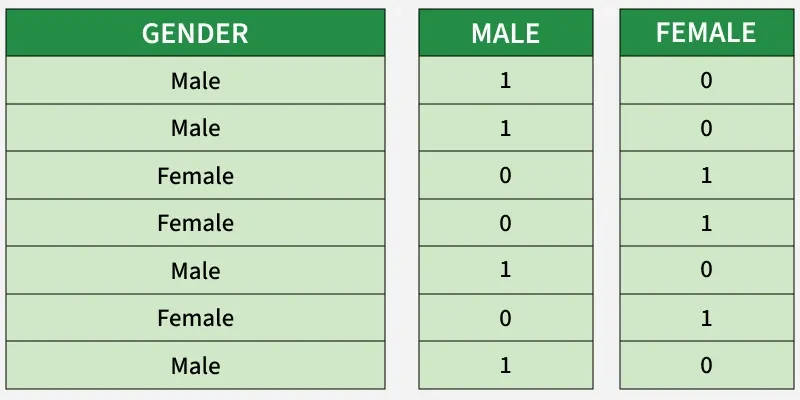
In multiple regression model we may encounter categorical data such as gender (male/female), location (urban/rural), etc. Since regression models require numerical inputs then categorical data must be transformed into a usable form. This is where Dummy Variables used. These are binary variables (0 or 1) that represent the presence or absence of each category. For example:

• Male: 1 if male, 0 otherwise
• Female: 1 if female, 0 otherwise

In the case of multiple categories we create a dummy variable for each category excluding one to avoid multicollinearity. This process is called one-hot encoding which converts categorical variables into a numerical format suitable for regression models.

Multicollinearity in Multiple Linear Regression

Multicollinearity arises when two or more independent variables are highly correlated with each other. This can make it difficult to find the individual contribution of each variable to the dependent variable.

To detect multicollinearity we can use:

1. Correlation Matrix: A correlation matrix helps to find relationships between independent variables. High correlations (close to 1 or -1) suggest multicollinearity.
2. VIF (Variance Inflation Factor): VIF quantifies how much the variance of a regression coefficient increases if predictors are correlated. A high VIF typically above 10 indicates multicollinearity.

Assumptions of Multiple Regression Model

Similar to simple linear regression we have some assumptions in multiple linear regression which are as follows:

1. Linearity: Relationship between dependent and independent variables should be linear.
2. Homoscedasticity: Variance of errors should remain constant across all levels of independent variables.
3. Multivariate Normality: Residuals should follow a normal distribution.
4. No Multicollinearity: Independent variables should not be highly correlated.

Implementation of Multiple Linear Regression Model

We will use the California Housing dataset which includes features such as median income, average rooms and the target variable, house prices.

Step 1: Importing Libraries

We will be using numpy, pandas, matplotlib and scikit learn for this.

Step 2: Loading Dataset

• Load the California Housing dataset from sklearn.datasets.
• Dataset contains features such as median income, average rooms stored in X and the target i.e house prices is stored in y.

Step 3: Selecting Features for Visualization

Choose two features MedInc (median income) and AveRooms (average rooms) to simplify visualization in two dimensions.

Step 4: Train-Test Split

We will use 80% data for training and 20% for testing.

Step 5: Initializing and Training Model

Create a multiple linear regression model using LinearRegression from scikit-learn and train it on the training data.

Step 6: Finding Intercept and Slopes

After training the model, we can access the intercept and coefficients of the regression equation.

• model.intercept_ : β₀ (intercept)
• model.coef_ : β₁, β₂ (slopes of MedInc and AveRooms)

Output:

Intercept: 0.5972677793933272

Coefficients: [ 0.43626089 -0.04017161]

Step 7: Making Predictions

Using the trained model to predict house prices on the test data.

Step 8: Visualizing Best- Fit Line in 3D

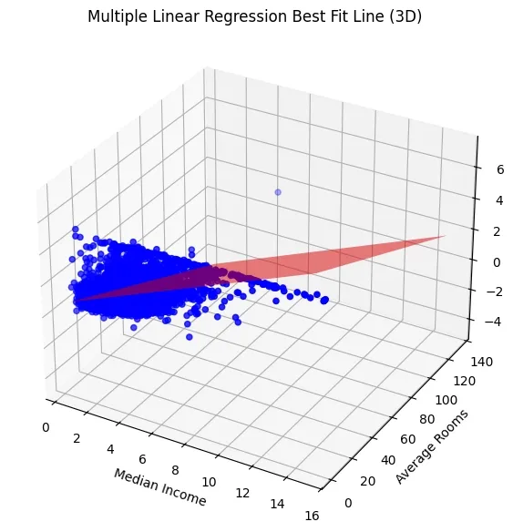
Plot a 3D graph where blue points represent actual house prices based on MedInc and AveRooms and the red surface shows the best-fit plane predicted by the model. This visualization helps us to understand how these two features influence the predicted house prices.

Output:

Multiple Linear Regression effectively captures how several factors together influence a target variable which helps in providing a practical approach for predictive modeling in real-world scenarios. 

You can download the complete source code from here.