Chi-square test in Data Science & Data Analytics

Chi-Square test helps us determine if there is a significant relationship between two categorical variables. It is a non-parametric statistical test meaning it doesn’t follow normal distribution.

The Chi-square test compares the observed frequencies (actual data) to the expected frequencies (what we would expect if there was no relationship). This helps identify which features are important for predicting the target variable in machine learning models.

Formula for Chi-square test

Chi-square statistic is calculated as:

where,

• c is degree of freedom
• is the observed frequency in cell
• is the expected frequency in cell

Often used with non-normally distributed data. Before we jump into calculations. let's understand some important terms:

• Observed Values (O): Actual counts from the data.
• Expected Values (E): Counts expected if variables are independent.
• Contingency Table: A table showing counts of two categorical variables.
• Degrees of Freedom (df): Number of independent values, helps find critical values.

Types of Chi-Square test

The two main types are the chi-square test for independence and the chi-square goodness-of-fit test.

1. Chi-Square Test for Independence: This test is used whether there is a significant relationship between two categorical variables.

• This test is applied when we have counts of values for two nominal or categorical variables.
• To conduct this test two requirements must be met: independence of observations and a relatively large sample size.
• We test if shopping preference (Electronics, Clothing, Books) is related to payment method (Credit Card, Debit Card, PayPal). The null hypothesis assumes no relationship between them.

2. Chi-Square Goodness-of-Fit Test:The Chi-Square Goodness-of-Fit test is used to check if a variable follows a specific expected pattern or distribution.

• This test is used with counts of categorical data to see if the observed values match what we expect based on a hypothesis. It helps determine if the data represents the whole population well.
• For example, when testing if a six-sided die is fair, the null hypothesis assumes each face has an equal chance of landing face up meaning the die is unbiased and all sides occur equally often.

Steps to perform Chi-square test

Step 1: Define Your Hypotheses

• Null Hypothesis (H₀): The two variables are independent (no relationship).
• Alternative Hypothesis (H₁): The two variables are related (there is a relationship).

Step 2: Create a Contingency Table: This is simply a table that displays the frequency distribution of the two categorical variables.

Step 3: Calculate Expected Values: To find the expected value for each cell use this formula:

Step 4: Compute the Chi-Square Statistic: Now use the Chi-Square formula:

where:

• O_i = Observed value
• E_i = Expected value

If the observed and expected values are very different the Chi-Square value will be high which indicate a strong relationship.

Step 5: Compare with the Critical Value:

• If > critical value → Reject H₀ (There is a relationship).
• If < critical value → Fail to reject H₀ (No relationship).

Uses of the Chi-Square Test

The Chi-Square Test helps us find relationships or differences between categories. Its main uses are:

1. Feature Selection in Machine Learning: It helps decide if a categorical feature (like color or product type) is important for predicting the target (like sales or satisfaction), improving model performance.
2. Testing Independence: It checks if two categorical variables are related or independent. For example, whether age or gender affects product preferences.
3. Assessing Model Fit: It helps check if a model’s predicted categories match the actual data, which is useful to improve classification models.

Example: Income Level vs Subscription Status

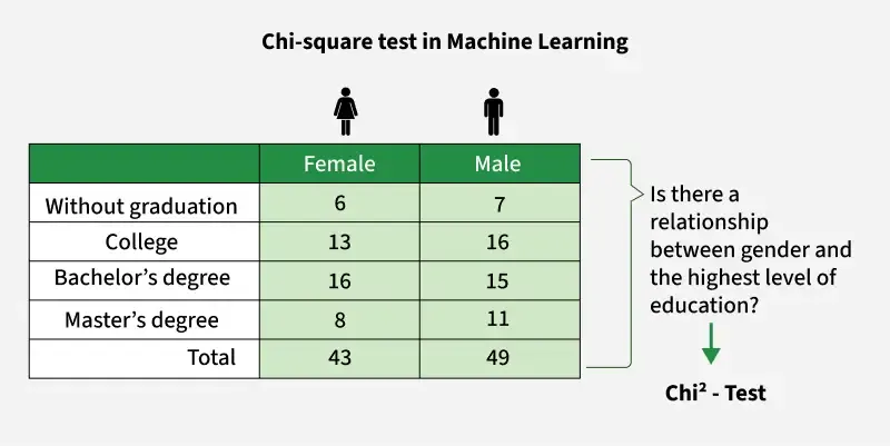
Let us examine a dataset with features including "income level" (low, medium, high) and "subscription status" (subscribed, not subscribed) indicate whether a customer subscribed to a service. The goal is to determine if this feature is relevant for predicting subscription status.

Step 1: Make Hypothesis

• Null hypothesis: No significant association between features
• Alternate Hypothesis: There is a significant association between features.

Step 2: Contingency table

Step 3: Now calculate the expected frequencies

For example the expected frequency for "Low Income" and "Subscribed" would be:

• As Total count for each row is 70 and each column is 70 and Total number of observations are 140.
• Low Income, subscribed=

Similarly we can find expected frequencies for other aspects as well:

Step 4: Calculate the Chi-Square Statistic

Let's summarize the observed and expected values into a table and calculate the Chi-Square value:

Now using the formula specified in equation 1 we can get our chi-square statistic values in the following manner:

Step 5: Degrees of Freedom

Step 6: Interpretations

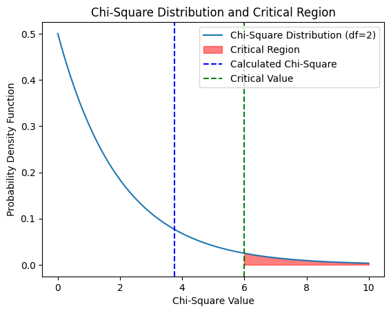
Now compare the calculated alue (6.462) with the critical value for 2 degrees of freedom. The critical value can be obtained either from a standard Chi-square distribution table or by using Python’s stats.chi2.ppf() function. If the calculated is greater than the critical value, then we reject the null hypothesis.

Before its implementation we should have some basic knowledge about numpy, matplotlib and scipy.

Output:

5.991464547107979

For df = 2 and significance level , the critical value is 5.991.

• Since 6.462 > 5.991, we reject the null hypothesis.
• Conclusion: There is a significant association between income level and subscription status.

Visualizing Chi-Square Distribution

Output:

In this example The green dashed line represents the critical value the threshold beyond which you would reject the null hypothesis.

• The red dashed line represents the critical value (5.991) for a significance level of 0.05 with 2 degrees of freedom.
• The shaded area to the right of the critical value represents the rejection region.

If the calculated Chi-Square statistic falls within this shaded area then you would reject the null hypothesis.