Normal Distribution in Data Science

The Normal Distribution (also called the Gaussian or Bell-shaped Distribution) is one of the most commonly used probability distributions in statistics. It is symmetric around the mean and forms the characteristic bell-shaped curve.

• It plays an essential role in statistics, especially in the Central Limit Theorem (CLT).
• Most values cluster near the mean and the probability decreases as we move away from it.

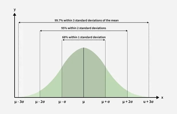
It can be observed in the above image that the distribution is symmetric about its center which is the mean (0 in this case). This makes the probability of events at equal deviations from the mean equally probable. The density is highly centered around the mean which translates to lower probabilities for values away from the mean.

Probability Density Function (PDF)

The PDF of the normal distribution gives the likelihood of a continuous random variable taking a specific value. The formula is:

where:

• (mu) is the mean (center of the distribution).
• (sigma) is the standard deviation (spread).
• is the value for which we calculate the probability.

To simplify this formula, we use the z-score, which tells us how many standard deviations a value is from the mean:

A larger z-score means the value is farther from the mean, giving a smaller probability due to the negative exponent. Values near the mean have higher probabilities.

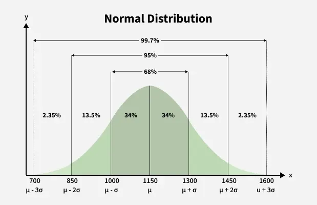
This behavior follows the 68–95–99.7 rule:

• 68% of values lie within 1 standard deviation from the mean,
• 95% lie within 2 standard deviations and
• 99.7% lie within 3 standard deviations.

The figure given below shows this rule:

Expectation (E[X]), Variance and Standard Deviation

The expectation or expected value of a random variable gives us a measure of the "center" of the distribution. For a normally distributed random variable with parameters (mean) and (variance), the expectation is calculated by integrating the product of the random variable and its probability density function (PDF) over all possible values.

Mathematically, the expected value is:

For the normal distribution, the formula becomes:

We can simplify this by breaking it into two parts:

• The first part involves integrating which is symmetric about the mean and its result is zero because the distribution is symmetric.
• The second part involves multiplying the mean by the total probability which equals 1 (since the area under the normal curve is always 1).

Thus we find:

This tells us that the expected value of a normal distribution is simply the mean .

Variance and Standard Deviation

The variance of a normal distribution is the square of the standard deviation denoted as . It measures how spread out the values of the distribution are from the mean.

The standard deviation is simply the square root of the variance:

Standard Normal Distribution

In the General Normal Distribution, if the Mean is set to 0 and the Standard Deviation is set to 1 then resulting distribution is called the Standard Normal Distribution. The formula for the Probability Density Function (PDF) of the standard normal distribution is:

where:

The Standard Normal Distribution is symmetric around the mean and its PDF defines the shape of the bell curve.

Cumulative Distribution Function (CDF)

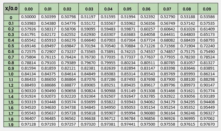
1. The Cumulative Distribution Function (CDF) of the normal distribution does not have a closed-form expression. As a result, precomputed values from standard normal tables are used to find cumulative probabilities. These tables specifically provide cumulative probabilities for the standard normal distribution.

2. For a general normal distribution, the first step is to standardize the distribution by converting it into a z-score. Once standardized, the cumulative probability is calculated using the standard normal distribution tables.

3. This process has two key benefits:

• Only one table is needed to calculate probabilities for all normal distributions regardless of the specific mean and standard deviation.
• The table size is manageable containing 40 to 50 rows and 10 columns.

This is consistent with the 68–95–99.7 rule, which states that 99.7% of values lie within ±3 standard deviations of the mean. Therefore, probabilities beyond x = μ+ 3σ become extremely small and are treated as approximately zero

Example: Finding Probabilities

Problem: Suppose that the current measurements in a strip of wire are assumed to follow a normal distribution with a mean of 10 milliamperes and a variance of four milliamperes ² . What is the probability that a measurement exceeds 13 milliamperes?

Solution

1. Let X denote the current in milliamperes. We are tasked with finding P (X > 13).

2. Standardize X by converting it to a z-score:

3. Now P(X > 13) becomes equivalent to P(Z > 1.5) in the standard normal distribution.

4. From the standard normal table, find the value of 

5. So 

Thus the probability that the current exceeds 13 milliamperes is approximately 0.06681 or 6.7%.

Implementation of Normal Distribution in Python

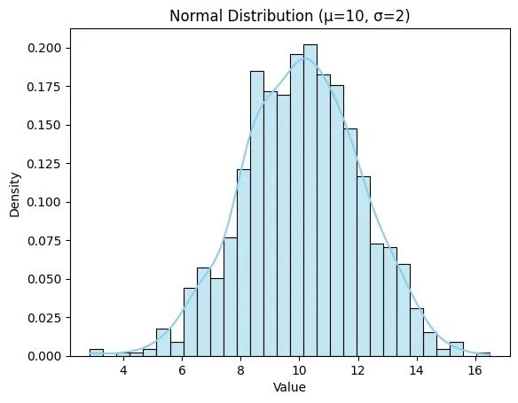
Here we will be using Numpy, Matplotlib and Seaborn libraries for the implementation.

Output:

Applications of Normal Distribution

The normal distribution is incredibly versatile and is used across a variety of fields:

1. Scientific Research: Measurement errors are normally distributed helps in making this distribution important in experimental design and hypothesis testing.
2. Finance: In stock market analysis, returns of stock prices follow a normal distribution. This helps in risk assessment and portfolio optimization.
3. Engineering: Manufacturing processes such as the dimensions of parts produced can be modeled using normal distribution.
4. Psychometrics: Test scores and IQ scores are assumed to follow a normal distribution helps in aiding in standardized testing and education.
5. Healthcare: Certain biological measurements (e.g blood pressure) tend to follow normal distributions which helps in identifying outliers or abnormal conditions.

Mastering the Standard Normal Distribution helps in the deeper understanding of probability which enables more accurate data interpretation and decision-making.