Geometric Distribution

A geometric distribution is a discrete probability distribution that gives the probability that the first success occurs on a specific trial in a sequence of independent Bernoulli trials, where each trial has two outcomes—success or failure—and the probability of success p remains constant across trials.

Geometric distributions are probability distributions that are based on three key assumptions.

• Trials are independent
• Each trial has one of two outcomes: success or failure
• For each trial, the probability of success, p, is constant across trials.

Example: Imagine you toss a fair coin repeatedly.

• Getting a head = success
• Getting a tail = failure

If you want to find the probability that the first head appears on the 4th toss, this situation follows a geometric distribution.

The geometric distribution is commonly used in various real-life circumstances. In the financial industry, it is used to estimate the financial rewards of making a given decision in a cost-benefit analysis.

Geometric Distribution Formulas

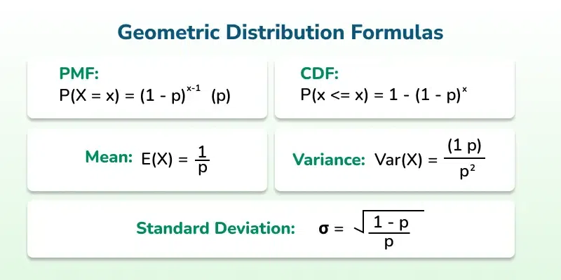
The geometric distribution is characterized by two important functions: the Probability Mass Function (PMF) and the Cumulative Distribution Function (CDF). These formulas help calculate the likelihood of achieving the first success after a certain number of trials. Below are the key formulas associated with the geometric distribution:

Geometric Distribution PMF

The likelihood that a discrete random variable, X, will be exactly identical to some value, x, is determined by the probability mass function.

P (X = x) = (1 - p)^{x -1}p

where, 0 < p ≤ 1.

Geometric Distribution CDF

The probability that a random variable, X, will assume a value that is less than or equal to x can be described as the cumulative distribution function of a random variable, X, that is assessed at a point, x. The distribution function is another name for it.

P(X ≤ x) = 1 - (1 - p)^x

Mean of Geometric Distribution

The geometric distribution's mean is also the geometric distribution's expected value. The weighted average of all values of a random variable, X, is the expected value of X.

E[X] = 1 / p

Variance of Geometric Distribution

Variance is a measure of dispersion that examines how far data in a distribution is spread out about the mean.

Var[X] = (1 - p) / p²

Standard Deviation of Geometric Distribution

The square root of the variance can be used to calculate the standard deviation. The standard deviation also indicates how far the distribution deviates from the mean.

S.D. = √VAR[X]

S.D. = √1 - p / p

Related Articles:

• Probability Theory
• Binomial Distribution
• Negative Binomial Distribution
• Probability Distribution Function

Sample Problems on Geometric Distribution

Problem 1: If a patient is waiting for a suitable blood donor and the probability that the selected donor will be a match is 0.2, then find the expected number of donors who will be tested till a match is found, including the matched donor.

Solution:

Given,
p = 0.2
E[X] = 1 / p 
= 1 / 0.2 
= 5

The expected number of donors who will be tested till a match is found is 5 

Problem 2: Suppose you are playing a game of darts. The probability of success is 0.4. What is the probability that you will hit the bullseye on the third try?

Solution:

Given,
p = 0.4
P(X = x) = (1 - p)^{x - 1}p
P(X = 3) = (1 - 0.4)^{3 - 1}(0.4)
P(X = 3) = (0.6)²(0.4) 
= 0.144

The probability that you will hit the bullseye on the third try is 0.144

Problem 3: A light bulb manufacturing factory finds 3 in every 60 light bulbs defective. What is the probability thatthe first defective light bulb with be found when the 6th one is tested?

Solution:

Given,
p = 3 / 60 = 0.05
P(X = x) = (1 - p)^{x - 1}p
P(X = 6) = (1 - 0.05)^{6 - 1}(0.05)
P(X = 6) = (0.95)⁵(0.05)
P(X = 6) = 0.0386

The probability that the first defective light bulb is found on the 6th trial is 0.0368

Problem 4: Find the probability density of the geometric distribution if the value of p is 0.42; x = 1,2,3, and also calculate the mean and variance.

Solution:

Given that p = 0.42 and the value of x = 1, 2, 3

The formula of probability density of geometric distribution is

P(x) = p (1 - p) ^x-1; x = 1, 2, 3
P(x) = 0; otherwise
P(x) = 0.42 (1 - 0.42)
P(x) = 0; Otherwise

Mean= 1/p
= 1/0.42
= 2.380

Variance = 1 - p/p²
= 1 - 0.42 /(0.42)²
= 3.287

Problem 5: If the probability of breaking the pot in the pool is 0.4, find the number of breaks before success and the corresponding variance and standard deviation.

Solution:

Here,
X ∼ geo(0.4)

Hence,
e(x) = 1/0.4 = 2.5
Var(x) = 0.6/0.4²
= 3.75

Hence, standard deviation ( σ) = 1.94