Sampling Distribution

Sampling distribution is essential in various aspects of real life, essential in inferential statistics. A sampling distribution represents the probability distribution of a statistic (such as the mean or standard deviation) that is calculated from multiple samples of a population. It helps us to understand how a statistic varies across different samples and is crucial for making inferences about the population.

Sampling distribution is the probability distribution of a statistic based on random samples of a given population. It is also know as finite distribution.

In this article, we will discuss the Sampling Distribution in detail and its types, along with examples, and go through some practice questions, too.

Important Terminologies in Sampling Distribution

Some important terminologies related to sampling distribution are given below:

• Statistic: Summary value from a sample (e.g., mean, median).
• Parameter: Summary value from a population.
• Sample: A subset of a population.
• Population: The entire group being studied.
• Sampling Distribution: Distribution of a statistic across many samples.
• Central Limit Theorem (CLT): Sample means follow a normal distribution as the sample size increases.
• Standard Error: Standard deviation of the sampling distribution.
• Bias: Systematic error causing deviation from the true value.
• Confidence Interval: Range likely to contain the population parameter.
• Sampling Method: How samples are chosen (random, stratified, etc.).
• Inferential Statistics: Concluding a population from samples.
• Hypothesis Testing: Making decisions about population parameters using sample data.

Factors Influencing Sampling Distribution

The variability of a sampling distribution is measured by standard error or population variance, depending on the context and the type of inference required. Both measure how spread out the data is around the mean.

Main factors influencing the variability of a sampling distribution are:

1. Number Observed in a Population: The symbol for this variable is "N." It is the measure of observed activity in a given group of data.
2. Number Observed in Sample: The symbol for this variable is "n." It is the measure of observed activity in a random sample of data that is part of the larger grouping.
3. Method of Choosing Sample: How you chose the samples can account for variability in some cases.

Types of Distributions

3 main types of sampling distributions are:

• Sampling Distribution of Mean
• Sampling Distribution of Proportion
• T-Distribution

Sampling Distribution of Mean

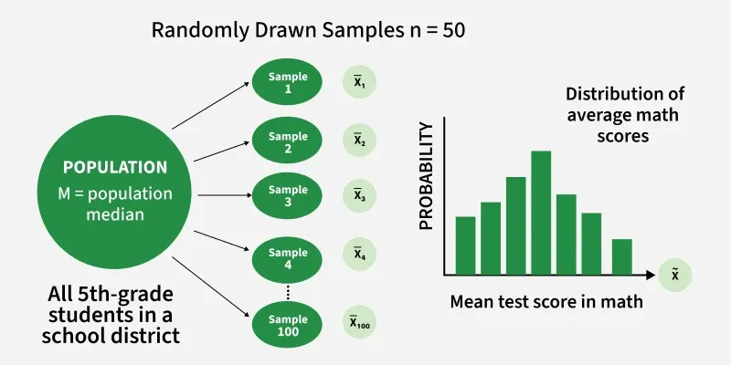
The sampling distribution of the mean refers to the probability distribution of sample means that you get by repeatedly taking samples (of the same size) from a population and calculating the mean of each sample.

Key concepts of Sampling Distribution of Mean

• Population Mean (μ): The average of the entire population.
• Sample Mean (x̄): The average of a sample taken from the population.
• Sampling Distribution of the Mean: If you take multiple samples and plot their means, that plot will form the sampling distribution of the mean.

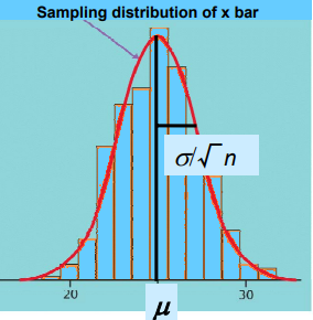
For any population with mean µ and standard deviation σ:

• Mean, or center of the sampling distribution of x̄, is equal to the population mean, µ.

= µ

There is no tendency for a sample mean to fall systematically above or below µ, even if the distribution of the raw data is skewed. Thus, the mean of the sampling distribution is an unbiased estimate of the population mean µ.

• Standard deviation of the sampling distribution is σ/√n, where n is the sample size.

= σ/√n

Where

• - Standard Deviation of Sampling Deviation
• σ - Population Standard Deviation
• n - Sample size
  

  👁 samp-dist-type-12
  

Sampling Distribution of Proportion

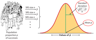
Sampling distribution of a proportion focuses on proportions in a population. Here, you select samples and calculate their corresponding proportions. The means of the sample proportions from each group represent the proportion of the entire population.

The formula for the sampling distribution of a proportion (often denoted as p̂) is:

p̂ = x/n

Where:

• p̂ is the Sample Proportion
• x is the Number of "successes" or occurrences of the Event of Interest in the Sample
• n is Sample Size

This formula calculates the proportion of occurrences of a certain event (e.g., success, positive outcome) within a sample.

T-Distribution

Sampling distribution involves a small population or a population about which you don't know much. It is used to estimate the mean of the population and other statistics such as confidence intervals, statistical differences, and linear regression. T-distribution uses a t-score to evaluate data that wouldn't be appropriate for a normal distribution.

The formula for the t-score, denoted as t, is:

t = [x - μ] / [s /√(n)]

Where:

• x is the Sample Mean
• μ is Population Mean (or an estimate of it)
• s is the Sample Standard Deviation
• n is Sample Size

This formula calculates the difference between the sample mean and the population mean, scaled by the standard error of the sample mean. The t-score helps to assess whether the observed difference between the sample and population means is statistically significant.

Solved Examples of Sampling Distribution

Example 1: Mean and standard deviation of the tax value of all vehicles registered in a certain state are μ=$13,525 and σ=$4,180. Suppose random samples of size 100 are drawn from the population of vehicles.
Find

• mean μ_x̄
• standard deviation σ_x̄ of the sample mean x̄

Solution:

Since n = 100, the formulas yield

μ_x̄ = μ = $13,525

σ_x̄ = σ / √n = $4180 / √100

σ_x̄ =$418

Example 2: A prototype automotive tire has a design life of 38,500 miles with a standard deviation of 2,500 miles. Five such tires are manufactured and tested. On the assumption that the actual population mean is 38,500 miles and the actual population standard deviation is 2,500 miles, find the probability that the sample mean will be less than 36,000 miles. Assume that the distribution of lifetimes of such tires is normal.

Solution:

Here, we will assume and use units of thousands of miles.

Then sample mean x̄ has

• Mean: μ_x̄ = μ = 38.5
• Standard Deviation: σ_x̄ = σ/√n = 2.5/√5 = 1.11803

Since the population is normally distributed, so is x̄, hence,

P (X < 36) = P(Z < {36 - μ_x̄}/σ_x̄)

P (X < 36) = P(Z < {36 - 38.5}/1.11803)

P (X < 36) = P(Z < -2.24)

P(X < 36) = 0.0125

Therefore, if the tires perform as designed then there is only about a 1.25% chance that the average of a sample of this size would be so low.

Practice Questions on Sample Distribution

Question 1: Random samples of size 225 are drawn from a population with a mean of 100 and a standard deviation of 20. Find the mean and standard deviation of the sample mean.

Question 2: Random samples of size 64 are drawn from a population with a mean of 32 and a standard deviation of 5. Find the mean and standard deviation of the sample mean.

Question 3: A population has a mean of 75 and a standard deviation of 12.

1. Random samples of size 121 are taken. Find the mean and standard deviation of the sample mean.
2. How would the answers to part
3. Change if the size of the samples were 400 instead of 121?

Question 4: A population has a mean of 5.75 and a standard deviation of 1.02.

1. Random samples of size 81 are taken. Find the mean and standard deviation of the sample mean.
2. How would the answers to part
3. Change if the size of the samples were 25 instead of 81?

Question 5: The Numerical population of grade point averages at a college has a mean of 2.61 and a standard deviation of 0.5. If a random sample of size 100 is taken from the population, what is the probability that the sample mean will be between 2.51 and 2.71?

Question 6: Random samples of size 1,600 are drawn from a population in which the proportion with the characteristic of interest is 0.05. Decide whether or not the sample size is large enough to assume that the sample proportion is normally distributed.