 |
VOOZH | about |
|
VOOZH | about |
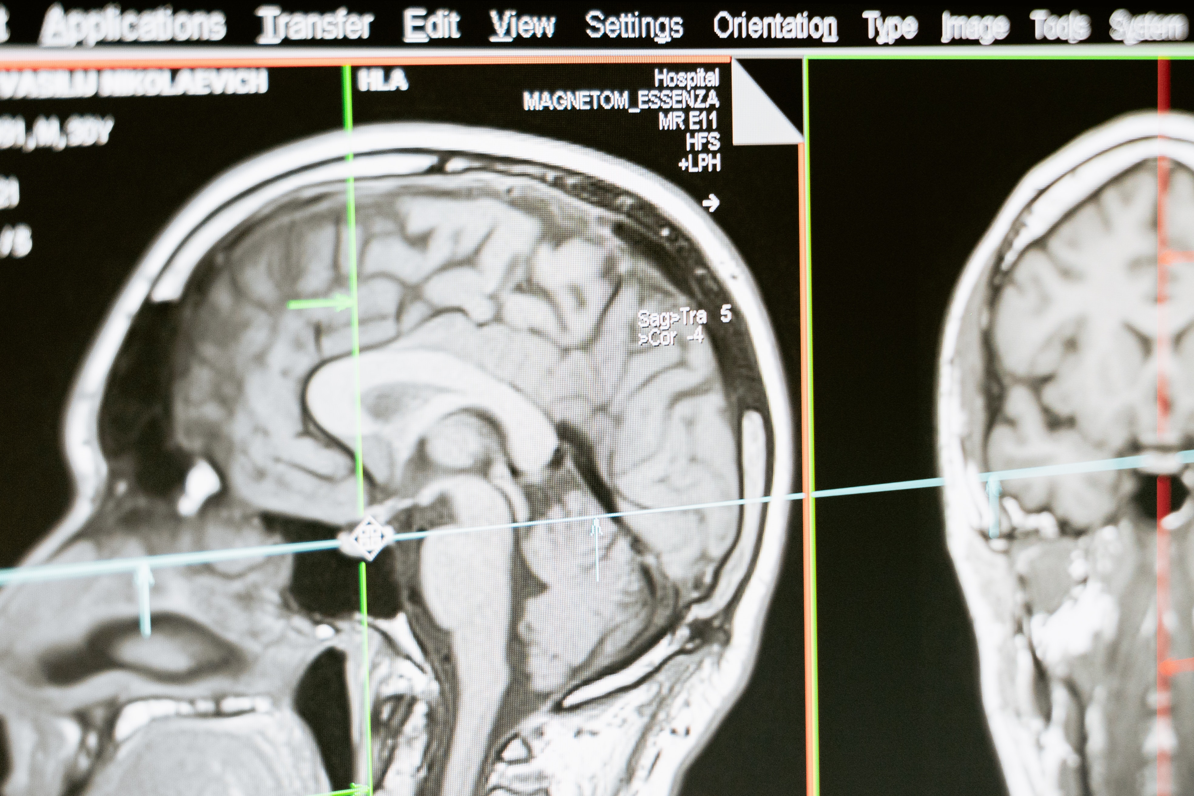
Photo by MART PRODUCTION from Pexels
To predict and localize brain tumors through image segmentation from the MRI dataset available in Kaggle.
I’ve divided this article into a series of two parts as we are going to train two deep learning models for the same dataset but the different tasks.
The model in this part is a classification model that will detect tumors from the MRI image and then if a tumor exists, we will further localize the segment of the brain having a tumor in the next part of this series.
Deep Learning
I’ll try to explicate every part thoroughly but in case you find any difficulty, let me know in the comment section. Let’s head into the implementation part using python.
Dataset: https://www.kaggle.com/mateuszbuda/lgg-mri-segmentation
import pandas as pd
import numpy as np
import seaborn as sns
import matplotlib.pyplot as plt
import cv2
from skimage import io
import tensorflow as tf
from tensorflow.python.keras import Sequential
from tensorflow.keras import layers, optimizers
from tensorflow.keras.applications.resnet50 import ResNet50
from tensorflow.keras.layers import *
from tensorflow.keras.models import Model
from tensorflow.keras.callbacks import EarlyStopping, ModelCheckpoint
from tensorflow.keras import backend as K
from sklearn.preprocessing import StandardScaler
%matplotlib inline
# data containing path to Brain MRI and their corresponding mask
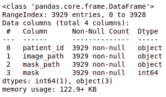
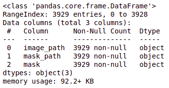
brain_df = pd.read_csv('/Healthcare AI Datasets/Brain_MRI/data_mask.csv')
brain_df.info()
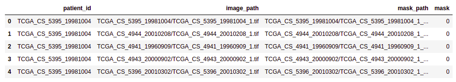
brain_df.head(5)
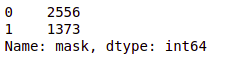
brain_df['mask'].value_counts()
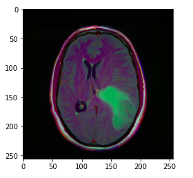
image = cv2.imread(brain_df.image_path[1301])
plt.imshow(image)
The image_path stores the path of the brain MRI so we can display the image using matplotlib.
Hint: The greenish portion in the above image can be considered as the tumor.
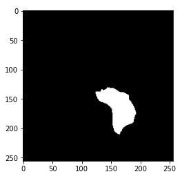
image1 = cv2.imread(brain_df.mask_path[1301])
plt.imshow(image1)
Now, you may have got the hint of what actually the mask is. The mask is the image of the part of the brain that is affected by a tumor of the corresponding MRI image. Here, the mask is of the above-displayed brain MRI.
cv2.imread(brain_df.mask_path[1301]).max()
Output: 255
The maximum pixel value in the mask image is 255 which indicates the white color.
cv2.imread(brain_df.mask_path[1301]).min()
Output: 0
The minimum pixel value in the mask image is 0 which indicates the black color.
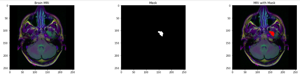
count = 0
fig, axs = plt.subplots(12, 3, figsize = (20, 50))
for i in range(len(brain_df)):
 if brain_df['mask'][i] ==1 and count <5:
 img = io.imread(brain_df.image_path[i])
 axs[count][0].title.set_text('Brain MRI')
 axs[count][0].imshow(img)

 mask = io.imread(brain_df.mask_path[i])
 axs[count][1].title.set_text('Mask')
 axs[count][1].imshow(mask, cmap = 'gray')

 img[mask == 255] = (255, 0, 0) #Red color
 axs[count][2].title.set_text('MRI with Mask')
 axs[count][2].imshow(img)
 count+=1

fig.tight_layout()
# Drop the patient id column
brain_df_train = brain_df.drop(columns = ['patient_id'])
brain_df_train.shape
You will get the size of the data frame in the output: (3929, 3)
brain_df_train['mask'] = brain_df_train['mask'].apply(lambda x: str(x))
brain_df_train.info()
As you can see, now each feature has the datatype as an object.
# split the data into train and test data from sklearn.model_selection import train_test_split train, test = train_test_split(brain_df_train, test_size = 0.15) |
Refer here for more information on ImageDataGenerator and the parameters in detail.
We will create a train_generator and validation_generator from train data and a test_generator from test data.
# create an image generator
from keras_preprocessing.image import ImageDataGenerator

#Create a data generator which scales the data from 0 to 1 and makes validation split of 0.15
datagen = ImageDataGenerator(rescale=1./255., validation_split = 0.15)

train_generator=datagen.flow_from_dataframe(
dataframe=train,
directory= './',
x_col='image_path',
y_col='mask',
subset="training",
batch_size=16,
shuffle=True,
class_mode="categorical",
target_size=(256,256))

valid_generator=datagen.flow_from_dataframe(
dataframe=train,
directory= './',
x_col='image_path',
y_col='mask',
subset="validation",
batch_size=16,
shuffle=True,
class_mode="categorical",
target_size=(256,256))

# Create a data generator for test images
test_datagen=ImageDataGenerator(rescale=1./255.)

test_generator=test_datagen.flow_from_dataframe(
dataframe=test,
directory= './',
x_col='image_path',
y_col='mask',
batch_size=16,
shuffle=False,
class_mode='categorical',
target_size=(256,256))
Now, we will learn the concept of Transfer Learning and ResNet50 Model which will be used for further training model.
Transfer Learning as the name suggests, is a technique to use the pre-trained models in your training. You can build your model on top of this pre-trained model. This is a process that helps you decrease the development time and increase performance.
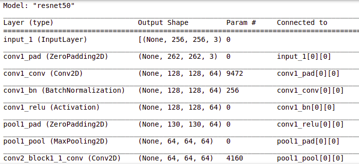
ResNet (Residual Network) is the ANN trained on the ImageNet dataset that can be used to train the model on top of it. ResNet50 is the variant of the ResNet model which has 48 Convolution layers along with 1 MaxPool and 1 Average Pool layer.
# Get the ResNet50 base model (Transfer Learning)
basemodel = ResNet50(weights = 'imagenet', include_top = False, input_tensor = Input(shape=(256, 256, 3)))
basemodel.summary()
You can view the layers in the resnet50 model by using .summary() as shown above.
# freeze the model weights
for layer in basemodel.layers:
 layers.trainable = False
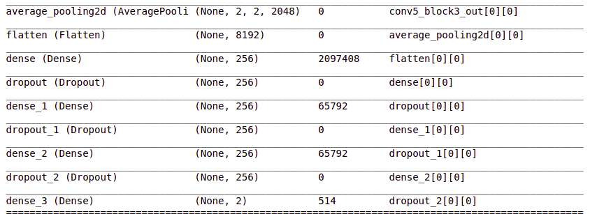
headmodel = basemodel.output
headmodel = AveragePooling2D(pool_size = (4,4))(headmodel)
headmodel = Flatten(name= 'flatten')(headmodel)
headmodel = Dense(256, activation = "relu")(headmodel)
headmodel = Dropout(0.3)(headmodel)
headmodel = Dense(256, activation = "relu")(headmodel)
headmodel = Dropout(0.3)(headmodel)
headmodel = Dense(256, activation = "relu")(headmodel)
headmodel = Dropout(0.3)(headmodel)
headmodel = Dense(2, activation = 'softmax')(headmodel)

model = Model(inputs = basemodel.input, outputs = headmodel)
model.summary()
These layers are added and you can see them in the summary.
# compile the model
model.compile(loss = 'categorical_crossentropy', optimizer='adam', metrics= ["accuracy"])
Read more about EarlyStopping here.
Read more about ModelCheckpoint parameters here.
# use early stopping to exit training if validation loss is not decreasing even after certain epochs
earlystopping = EarlyStopping(monitor='val_loss', mode='min', verbose=1, patience=20)

# save the model with least validation loss
checkpointer = ModelCheckpoint(filepath="classifier-resnet-weights.hdf5", verbose=1, save_best_only=True)
model.fit(train_generator, steps_per_epoch= train_generator.n // 16, epochs = 1, validation_data= valid_generator, validation_steps= valid_generator.n // 16, callbacks=[checkpointer, earlystopping])
# make prediction
test_predict = model.predict(test_generator, steps = test_generator.n // 16, verbose =1)

# Obtain the predicted class from the model prediction
predict = []
for i in test_predict:
 predict.append(str(np.argmax(i)))
predict = np.asarray(predict)
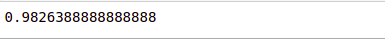
# Obtain the accuracy of the model
from sklearn.metrics import accuracy_score

accuracy = accuracy_score(original, predict)
accuracy
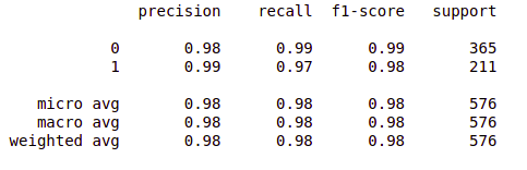
from sklearn.metrics import classification_report
report = classification_report(original, predict, labels = [0,1])
print(report)
So far so good!
Now, you can pat yourself as you have just completed the first part i.e., brain tumor detection. Now, we will head towards brain tumor segmentation in the second part of this series.
Brain Tumor Detection and Localization using Deep Learning: Part 2
Being a Data Science enthusiast, I write similar articles related to Machine Learning, Deep Learning, Computer Vision, and many more. Follow my medium account: https://medium.com/@mahishapatel to get updates about my articles.
Also, I’d love to connect with you on Linkedin: https://www.linkedin.com/in/mahisha-patel/
Your suggestions and doubts are welcomed here in the comment section. Thank you for reading my article!
GPT-4 vs. Llama 3.1 – Which Model is Better?
Llama-3.1-Storm-8B: The 8B LLM Powerhouse Surpa...
A Comprehensive Guide to Building Agentic RAG S...
Top 10 Machine Learning Algorithms in 2026
45 Questions to Test a Data Scientist on Basics...
90+ Python Interview Questions and Answers (202...
8 Easy Ways to Access ChatGPT for Free
Prompt Engineering: Definition, Examples, Tips ...
What is LangChain?
What is Retrieval-Augmented Generation (RAG)?
Hello, I couldn't find the dataset that you shared a link. It gives a different dataset from yours.
Edit
Resend OTP
Resend OTP in 45s