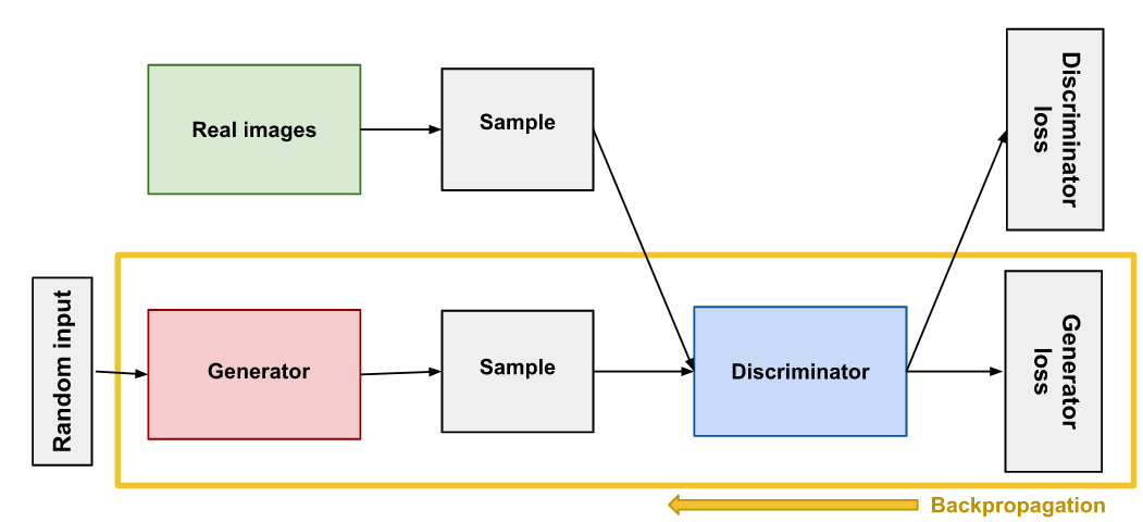
GANs are used for teaching a deep learning model to generate new data from that same distribution of training data. Invented by Ian Goodfellow in 2014 in the paper Generative Adversarial Nets. They are made up of two different models, a generatorand a discriminator. The generator produces synthetic or fake images which look like training images. The discriminator looks at an image and the output and checks if the image is real or fake. While training, the generator generates better fake images and fools the discriminator to believe that the generated image is a real image and the discriminator tries to become better at detection and classifying whether the image is real or fake.

👁 DCGAN 1

Source: https://developers.google.com/machine-learning/gan/generator

DCGAN

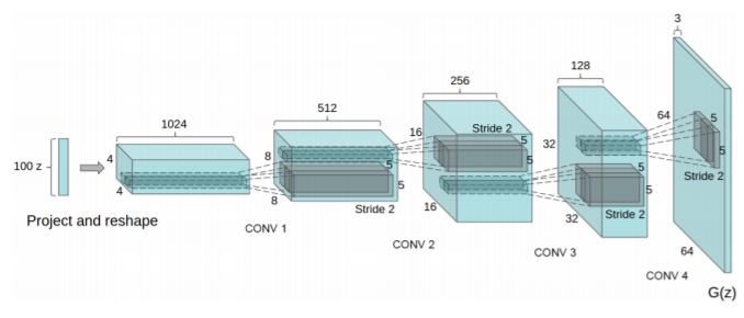
DCGAN uses convolutional and convolutional-transpose layers in the generator and discriminator, respectively. It was proposed by Radford et. al. in the paper Unsupervised Representation Learning With Deep Convolutional Generative Adversarial Networks. Here the discriminator consists of strided convolution layers, batch normalization layers, and LeakyRelu as activation function. It takes a 3x64x64 input image. The generator consists of convolutional-transpose layers, batch normalization layers, and ReLU activations. The output will be a 3x64x64 RGB image.

👁 DCGAN paper

Source: From the paper “Unsupervised Representation Learning With Deep Convolutional Generative Adversarial Networks”

Let’s implement DCGAN using celeba dataset, the dataset is available at https://drive.google.com/drive/folders/0B7EVK8r0v71pTUZsaXdaSnZBZzg. Download the data and extract it to the project directory or use the colab environment to access the data through google drive. Open the link and you will see img_align_celeba.zip, right-click and select the make a copy option, it will save a copy in the My drive section.

We will you colab environment to run our code. We can also set up locally.

First, we will get the dataset from the drive.

from google.colab import drive
drive.mount("/content/drive")

The above code will create a folder names drive in colab and you can see the dataset is in your desired path. Then we need to extract the zip file. Create a folder named dataset and extract the data to that folder

# Rename the file name from "Copy of img_align_celeba.zip" to "img_align_celeba.zip"
!unzip /content/drive/MyDrive/img_align_celeba.zip -d "/content/dataset"

Let’s import the required modules

from __future__ import print_function
import argparse
import os
import random
import torch
import torch.nn as nn
import torch.nn.parallel
import torch.backends.cudnn as cudnn
import torch.optim as optim
import torch.utils.data
import torchvision.datasets as dset
import torchvision.transforms as transforms
import torchvision.utils as vutils
import numpy as np
import matplotlib.pyplot as plt
import matplotlib.animation as animation
from IPython.display import HTML

Let’s define our inputs:

dataroot – the path to the root of the dataset folder.
workers – the number of worker threads for loading the data with the help of DataLoader
batch_size – the batch size used in training.
image_size – the spatial size of the images used for training.
nc – number of color channels in the input images.
nz – length of latent vector
ngf – relates to the depth of feature maps.
ndf – sets the depth of feature maps propagated through the discriminator
num_epochs – number of training epochs to run.
lr – learning rate for training.
beta1 – beta1 hyperparameter for Adam optimizers.
ngpu – number of GPUs available. 0 for cpu

dataroot = "/content/dataset"
workers = 2
batch_size = 128
image_size = 64
nc = 3
nz = 100
ngf = 64
ndf = 64
num_epochs = 5
lr = 0.0002
beta1 = 0.5
ngpu = 1

Here we will be using the ImageFolder dataset class, which requires a subdirectory in the dataset’s root folder. We can create the dataloader, visualize some of the training data.

dataset = dset.ImageFolder(root=dataroot,
 transform=transforms.Compose([
 transforms.Resize(image_size),
 transforms.CenterCrop(image_size),
 transforms.ToTensor(),
 transforms.Normalize((0.5, 0.5, 0.5), (0.5, 0.5, 0.5)),
 ]))
# Create the dataloader
dataloader = torch.utils.data.DataLoader(dataset, batch_size=batch_size,
 shuffle=True, num_workers=workers)
# Decide which device we want to run on
device = torch.device("cuda:0" if (torch.cuda.is_available() and ngpu > 0) else "cpu")
# Plot some training images
real_batch = next(iter(dataloader))
plt.figure(figsize=(8,8))
plt.axis("off")
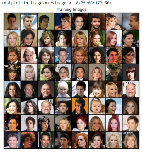
plt.title("Training Images")
plt.imshow(np.transpose(vutils.make_grid(real_batch[0].to(device)[:64], padding=2, normalize=True).cpu(),(1,2,0)))

The above code will display the training data.

👁 DCGAN show plot

A visual on the dataset

Weight Initialization

From the DCGAN paper, all model weights are initialized randomly from a Normal distribution with mean=0, standard_deviation=0.02. The initialized model will be given as input to the weights_init function and reinitializes all layers to meet weight initialization criteria.

def weights_init(m):
 classname = m.__class__.__name__
 if classname.find('Conv') != -1:
 nn.init.normal_(m.weight.data, 0.0, 0.02)
 elif classname.find('BatchNorm') != -1:
 nn.init.normal_(m.weight.data, 1.0, 0.02)
 nn.init.constant_(m.bias.data, 0)

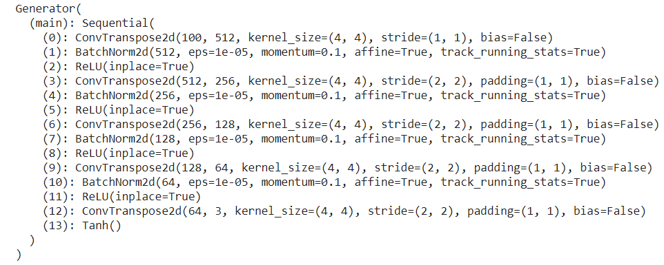
Now we can initialize our generator

# Generator Code
class Generator(nn.Module):
 def __init__(self, ngpu):
 super(Generator, self).__init__()
 self.ngpu = ngpu
 self.main = nn.Sequential(
 # input is Z, going into a convolution
 nn.ConvTranspose2d( nz, ngf * 8, 4, 1, 0, bias=False),
 nn.BatchNorm2d(ngf * 8),
 nn.ReLU(True),
 # state size. (ngf*8) x 4 x 4
 nn.ConvTranspose2d(ngf * 8, ngf * 4, 4, 2, 1, bias=False),
 nn.BatchNorm2d(ngf * 4),
 nn.ReLU(True),
 # state size. (ngf*4) x 8 x 8
 nn.ConvTranspose2d( ngf * 4, ngf * 2, 4, 2, 1, bias=False),
 nn.BatchNorm2d(ngf * 2),
 nn.ReLU(True),
 # state size. (ngf*2) x 16 x 16
 nn.ConvTranspose2d( ngf * 2, ngf, 4, 2, 1, bias=False),
 nn.BatchNorm2d(ngf),
 nn.ReLU(True),
 # state size. (ngf) x 32 x 32
 nn.ConvTranspose2d( ngf, nc, 4, 2, 1, bias=False),
 nn.Tanh()
 # state size. (nc) x 64 x 64
 )
 def forward(self, input):
 return self.main(input)

netG = Generator(ngpu).to(device)
# Handle multi-gpu if desired
if (device.type == 'cuda') and (ngpu > 1):
 netG = nn.DataParallel(netG, list(range(ngpu)))
netG.apply(weights_init)
# Print the model
print(netG)

👁 DCGAN netg

Output after executing above code

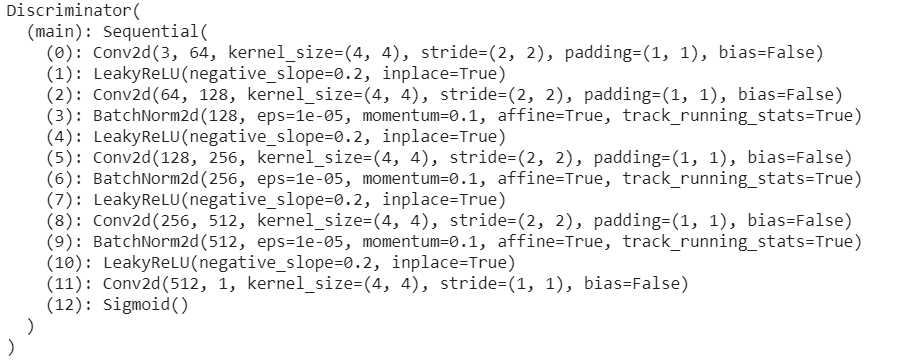
Then initializing the discriminator

class Discriminator(nn.Module):
 def __init__(self, ngpu):
 super(Discriminator, self).__init__()
 self.ngpu = ngpu
 self.main = nn.Sequential(
 # input is (nc) x 64 x 64
 nn.Conv2d(nc, ndf, 4, 2, 1, bias=False),
 nn.LeakyReLU(0.2, inplace=True),
 # state size. (ndf) x 32 x 32
 nn.Conv2d(ndf, ndf * 2, 4, 2, 1, bias=False),
 nn.BatchNorm2d(ndf * 2),
 nn.LeakyReLU(0.2, inplace=True),
 # state size. (ndf*2) x 16 x 16
 nn.Conv2d(ndf * 2, ndf * 4, 4, 2, 1, bias=False),
 nn.BatchNorm2d(ndf * 4),
 nn.LeakyReLU(0.2, inplace=True),
 # state size. (ndf*4) x 8 x 8
 nn.Conv2d(ndf * 4, ndf * 8, 4, 2, 1, bias=False),
 nn.BatchNorm2d(ndf * 8),
 nn.LeakyReLU(0.2, inplace=True),
 # state size. (ndf*8) x 4 x 4
 nn.Conv2d(ndf * 8, 1, 4, 1, 0, bias=False),
 nn.Sigmoid()
 )
 def forward(self, input):
 return self.main(input)

# Create the Discriminator
netD = Discriminator(ngpu).to(device)
# Handle multi-gpu if desired
if (device.type == 'cuda') and (ngpu > 1):
 netD = nn.DataParallel(netD, list(range(ngpu)))
netD.apply(weights_init)
# Print the model
print(netD)

👁 netd

Output after executing the above code

No, we initialize loss function and optimizer, we are going to use BCE loss function and Adam optimizer for generator and discriminator.

criterion = nn.BCELoss()
fixed_noise = torch.randn(64, nz, 1, 1, device=device)
# Establish convention for real and fake labels during training
real_label = 1.
fake_label = 0.
# Setup Adam optimizers for both G and D
optimizerD = optim.Adam(netD.parameters(), lr=lr, betas=(beta1, 0.999))
optimizerG = optim.Adam(netG.parameters(), lr=lr, betas=(beta1, 0.999))

Now let’s start the training of our DCGAN model. Training GANs is an art form itself, as incorrect hyperparameter settings lead to mode collapse. So play with different hyperparameters to obtain better results.

img_list = []
G_losses = []
D_losses = []
iters = 0
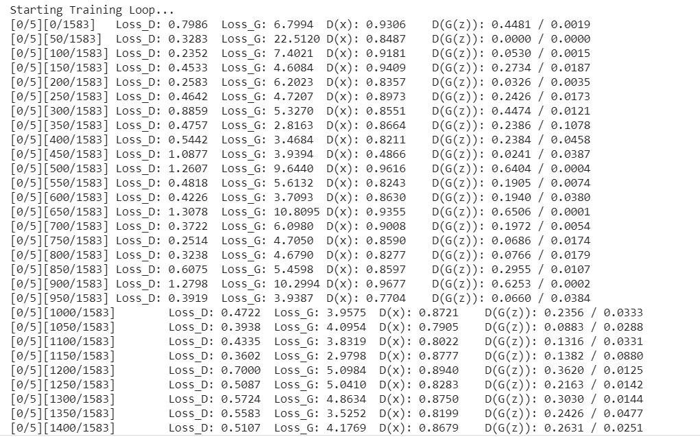
print("Starting Training Loop...")
# For each epoch
for epoch in range(num_epochs):
 # For each batch in the dataloader
 for i, data in enumerate(dataloader, 0):
 ############################
 # (1) Update D network: maximize log(D(x)) + log(1 - D(G(z)))
 ###########################
 ## Train with all-real batch
 netD.zero_grad()
 # Format batch
 real_cpu = data[0].to(device)
 b_size = real_cpu.size(0)
 label = torch.full((b_size,), real_label, dtype=torch.float, device=device)
 # Forward pass real batch through D
 output = netD(real_cpu).view(-1)
 # Calculate loss on all-real batch
 errD_real = criterion(output, label)
 # Calculate gradients for D in backward pass
 errD_real.backward()
 D_x = output.mean().item()
 ## Train with all-fake batch
 # Generate batch of latent vectors
 noise = torch.randn(b_size, nz, 1, 1, device=device)
 # Generate fake image batch with G
 fake = netG(noise)
 label.fill_(fake_label)
 # Classify all fake batch with D
 output = netD(fake.detach()).view(-1)
 # Calculate D's loss on the all-fake batch
 errD_fake = criterion(output, label)
 # Calculate the gradients for this batch, accumulated (summed) with previous gradients
 errD_fake.backward()
 D_G_z1 = output.mean().item()
 # Compute error of D as sum over the fake and the real batches
 errD = errD_real + errD_fake
 # Update D
 optimizerD.step()
 ############################
 # (2) Update G network: maximize log(D(G(z)))
 ###########################
 netG.zero_grad()
 label.fill_(real_label) # fake labels are real for generator cost
 # Since we just updated D, perform another forward pass of all-fake batch through D
 output = netD(fake).view(-1)
 # Calculate G's loss based on this output
 errG = criterion(output, label)
 # Calculate gradients for G
 errG.backward()
 D_G_z2 = output.mean().item()
 # Update G
 optimizerG.step()
 # Output training stats
 if i % 50 == 0:
 print('[%d/%d][%d/%d]tLoss_D: %.4ftLoss_G: %.4ftD(x): %.4ftD(G(z)): %.4f / %.4f'
 % (epoch, num_epochs, i, len(dataloader),
 errD.item(), errG.item(), D_x, D_G_z1, D_G_z2))
 # Save Losses for plotting later
 G_losses.append(errG.item())
 D_losses.append(errD.item())
 # Check how the generator is doing by saving G's output on fixed_noise
 if (iters % 500 == 0) or ((epoch == num_epochs-1) and (i == len(dataloader)-1)):
 with torch.no_grad():
 fake = netG(fixed_noise).detach().cpu()
 img_list.append(vutils.make_grid(fake, padding=2, normalize=True))
 iters += 1

The above code starts the training, It will take some time to run on GPU

👁 training

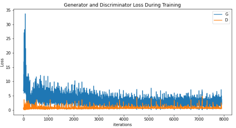
Let us plot the generator and discriminator losses

plt.figure(figsize=(10,5))
plt.title("Generator and Discriminator Loss During Training")
plt.plot(G_losses,label="G")
plt.plot(D_losses,label="D")
plt.xlabel("iterations")
plt.ylabel("Loss")
plt.legend()
plt.show()

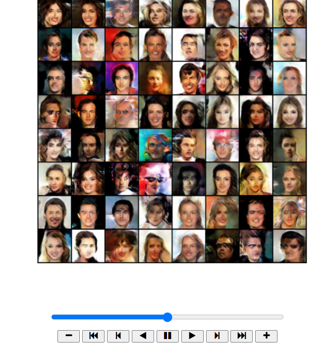
👁 generator and discriminator losses

Since we saved the generator’s output on the fixed_noise batch after every epoch. Now, we can visualize the training progression of the Generator with a little animation. Press the play button to visualize the training output.

fig = plt.figure(figsize=(8,8))
plt.axis("off")
ims = [[plt.imshow(np.transpose(i,(1,2,0)), animated=True)] for i in img_list]
ani = animation.ArtistAnimation(fig, ims, interval=1000, repeat_delay=1000, blit=True)
HTML(ani.to_jshtml())

👁 format

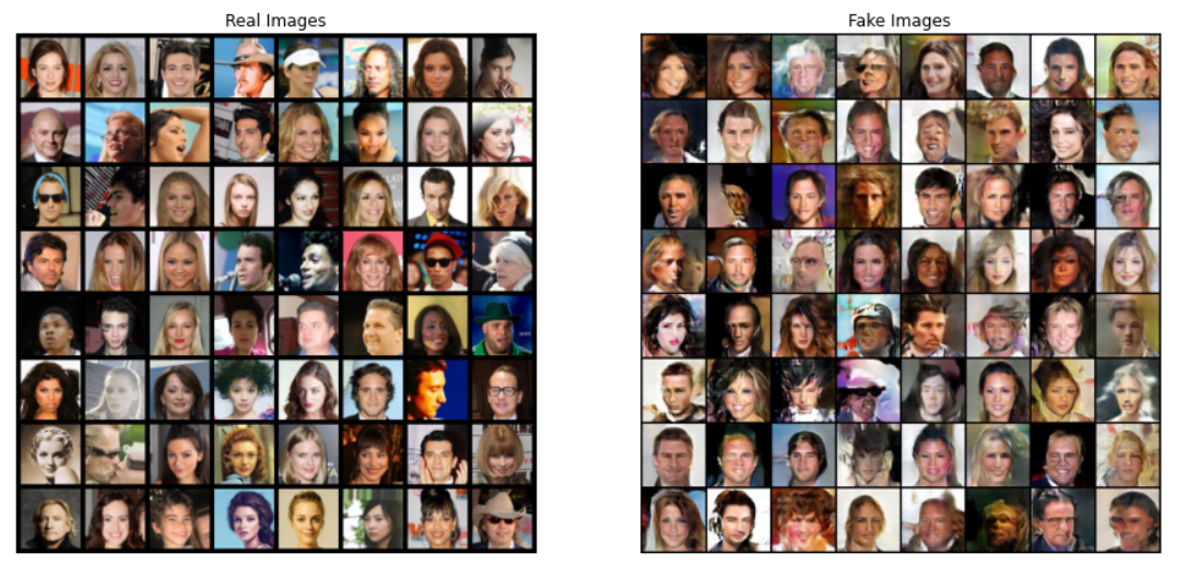
Finally, lets compare real images and fake images side by side.

real_batch = next(iter(dataloader))

# Plot the real images

plt.figure(figsize=(15,15))

plt.subplot(1,2,1)

plt.axis("off")

plt.title("Real Images")

plt.imshow(np.transpose(vutils.make_grid(real_batch[0].to(device)[:64], padding=5, normalize=True).cpu(),(1,2,0)))


# Plot the fake images from the last epoch

plt.subplot(1,2,2)

plt.axis("off")

plt.title("Fake Images")

plt.imshow(np.transpose(img_list[-1],(1,2,0)))

plt.show()

Below is the output.

👁 output

The colab file is available here

Reference:

https://pytorch.org/tutorials/beginner/dcgan_faces_tutorial.html

https://github.com/pytorch/tutorials/blob/master/beginner_source/dcgan_faces_tutorial.py

Thank You

The media shown in this article are not owned by Analytics Vidhya and are used at the Author’s discretion.

👁 Syed Abdul Gaffar

Syed Abdul Gaffar

I thrive on the thrill of the challenge, tackling complex problems and crafting innovative AI solutions that make a difference. Whether it's optimizing or building sustainable AI ecosystems, I believe in harnessing the power of AI for the greater good. Let's brainstorm, collaborate, and change the world, one byte at a time.

Advanced Computer Vision Image Image Analysis Project Python Python