Complete Guide On Complexity Analysis - Data Structure and Algorithms Tutorial

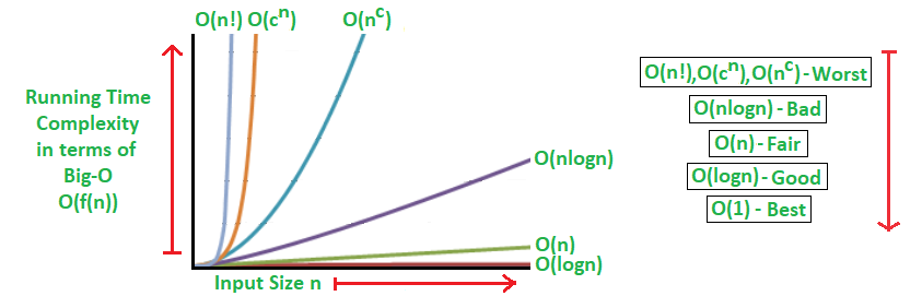
Complexity analysis is defined as a technique to characterise the time taken by an algorithm with respect to input size (independent from the machine, language and compiler). It is used for evaluating the variations of execution time on different algorithms.

What is the need for Complexity Analysis?

• Complexity Analysis determines the amount of time and space resources required to execute it.
• It is used for comparing different algorithms on different input sizes.
• Complexity helps to determine the difficulty of a problem.
• often measured by how much time and space (memory) it takes to solve a particular problem

Things to learn about Complexity Analysis

Asymptotic Notations in Complexity Analysis:

1. Big O Notation

Big-O notation represents the upper bound of the running time of an algorithm. Therefore, it gives the worst-case complexity of an algorithm. By using big O- notation, we can asymptotically limit the expansion of a running time to a range of constant factors above and below. It is a model for quantifying algorithm performance. 

O(g(n)) = { f(n): there exist positive constants c and n0 such that 0 ≤ f(n) ≤ cg(n) for all n ≥ n0 }

2. Omega Notation

Omega notation represents the lower bound of the running time of an algorithm. Thus, it provides the best-case complexity of an algorithm.
The execution time serves as a lower bound on the algorithm’s time complexity. It is defined as the condition that allows an algorithm to complete statement execution in the shortest amount of time.

Ω(g(n)) = { f(n): there exist positive constants c and n0 such that 0 ≤ cg(n) ≤ f(n) for all n ≥ n0 }
Note: Ω (g) is a set

3. Theta Notation

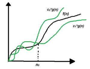
Theta notation encloses the function from above and below. Since it represents the upper and the lower bound of the running time of an algorithm, it is used for analyzing the average-case complexity of an algorithm. The execution time serves as both a lower and upper bound on the algorithm’s time complexity. It exists as both, the most, and least boundaries for a given input value.

Θ (g(n)) = {f(n): there exist positive constants c₁, c₂ and n₀ such that 0 ≤ c₁ * g(n) ≤ f(n) ≤ c₂ * g(n) for all n ≥ n₀}

4. Little ο asymptotic notation

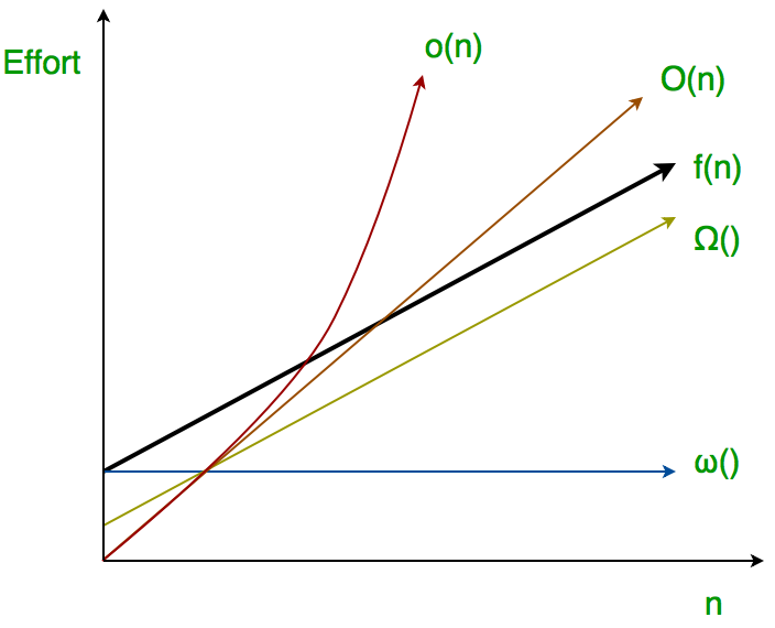
Big-Ο is used as a tight upper bound on the growth of an algorithm’s effort (this effort is described by the function f(n)), even though, as written, it can also be a loose upper bound. “Little-ο” (ο()) notation is used to describe an upper bound that cannot be tight. 

f(n) = o(g(n)) means lim  f(n)/g(n) = 0 n→∞ 

5. Little ω asymptotic notation

Let f(n) and g(n) be functions that map positive integers to positive real numbers. We say that f(n) is ω(g(n)) (or f(n) ∈ ω(g(n))) if for any real constant c > 0, there exists an integer constant n0 ≥ 1 such that f(n) > c * g(n) ≥ 0 for every integer n ≥ n0. 

if f(n) ∈ ω(g(n)) then, 

lim  f(n)/g(n) = ∞ 

n→∞ 

Note:  In most of the Algorithm we use Big-O notation, as it is worst case Complexity Analysis.

How to measure complexity?

The complexity of an algorithm can be measured in three ways:

1. Time Complexity

The time complexity of an algorithm is defined as the amount of time taken by an algorithm to run as a function of the length of the input. Note that the time to run is a function of the length of the input and not the actual execution time of the machine on which the algorithm is running on

To estimate the time complexity, we need to consider the cost of each fundamental instruction and the number of times the instruction is executed.

• If we have statements with basic operations like comparisons,return statements,assignments, and reading a variable. We can assume they take constant time each O(1).

Statement 1: int a=5; // reading a variable
statement 2; if( a==5) return true; // return statement
statement 3; int x= 4>5 ? 1:0; // comparison
statement 4; bool flag=true; // Assignment

This is the result of calculating the overall time complexity.

total time = time(statement1) + time(statement2) + ... time (statementN)

Assuming that n is the size of the input, let's use T(n) to represent the overall time and t to represent the amount of time that a statement or collection of statements takes to execute.

T(n) = t(statement1) + t(statement2) + ... + t(statementN); 

Overall, T(n)= O(1), which means constant complexity.

• For any loop, we find out the runtime of the block inside them and multiply it by the number of times the program will repeat the loop.

for (int i = 0; i < n; i++) {
   cout << "GeeksForGeeks" << endl;
}

For the above example, the loop will execute n times, and it will print "GeeksForGeeks"N number of times. so the time taken to run this program is:

T(N)= n *( t(cout statement))
 = n * O(1)
 =O(n), Linear complexity.

• For 2D arrays, we would have nested loop concepts, which means a loop inside a loop.

for (int i = 0; i < n; i++) {
   for (int j = 0; j < m; j++) {
       cout << "GeeksForGeeks" << endl;
   }
}

For the above example, the cout statement will execute n*m times, and it will print "GeeksForGeeks"N*M number of times. so the time taken to run this program is:

T(N)= n * m *(t(cout statement))
 = n * m * O(1)
 =O(n*m), Quadratic Complexity.

2. Space Complexity :

The amount of memory required by the algorithm to solve a given problem is called the space complexity of the algorithm. Problem-solving using a computer requires memory to hold temporary data or final result while the program is in execution. 

The space Complexity of an algorithm is the total space taken by the algorithm with respect to the input size. Space complexity includes both Auxiliary space and space used by input. 
Space complexity is a parallel concept to time complexity. If we need to create an array of size n, this will require O(n) space. If we create a two-dimensional array of size n*n, this will require O(n²) space.

In recursive calls stack space also counts.

Example:

int add (int n){
 if (n <= 0){
 return 0;
 }
 return n + add (n-1);
}
Here each call add a level to the stack :
1. add(4)
2. -> add(3)
3. -> add(2)
4. -> add(1)
5. -> add(0)
Each of these calls is added to call stack and takes up actual memory.
So it takes O(n) space.

However, just because you have n calls total doesn’t mean it takes O(n) space.

Look at the below function :

int addSequence (int n){
 int sum = 0;
 for (int i = 0; i < n; i++){
 sum += pairSum(i, i+1);
 }
 return sum;
}
int pairSum(int x, int y){
 return x + y;
}
There will be roughly O(n) calls to pairSum. However, those 
calls do not exist simultaneously on the call stack,
so you only need O(1) space.

3. Auxiliary Space :

The temporary space needed for the use of an algorithm is referred to as auxiliary space. Like temporary arrays, pointers, etc. 
It is preferable to make use of Auxiliary Space when comparing things like sorting algorithms. 
for example, sorting algorithms take O(n) space, as there is an input array to sort. but auxiliary space is O(1) in that case. 

How does Complexity affect any algorithm?

Time complexity of an algorithm quantifies the amount of time taken by an algorithm to run as a function of length of the input. While, the space complexity of an algorithm quantifies the amount of space or memory taken by an algorithm to run  as a function of the length of the input.

How to optimize the time and space complexity of an Algorithm?

Optimization means modifying the brute-force approach to a problem. It is done to derive the best possible solution to solve the problem so that it will take less time and space complexity. We can optimize a program by either limiting the search space at each step or occupying less search space from the start.

We can optimize a solution using both time and space optimization. To optimize a program,

1. We can reduce the time taken to run the program and increase the space occupied;
2. we can reduce the memory usage of the program and increase its total run time, or
3. we can reduce both time and space complexity by deploying relevant algorithms

Different types of Complexity exist in the program:

1. Constant Complexity

If the function or method of the program takes negligible execution time. Then that will be considered as constant complexity. 

Example:  The below program takes a constant amount of time.

Odd

2. Logarithmic Complexity:

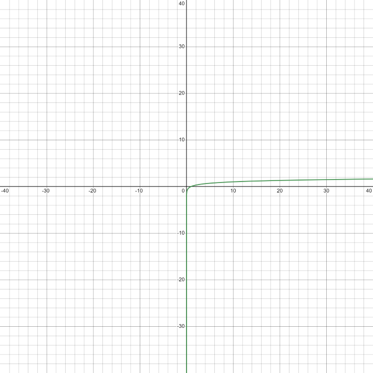
It imposes a complexity of O(log(N)). It undergoes the execution of the order of log(N) steps. To perform operations on N elements, it often takes the logarithmic base as 2. 

Example: The below program takes logarithmic complexity.

Element is present at index 3

3. Linear Complexity:

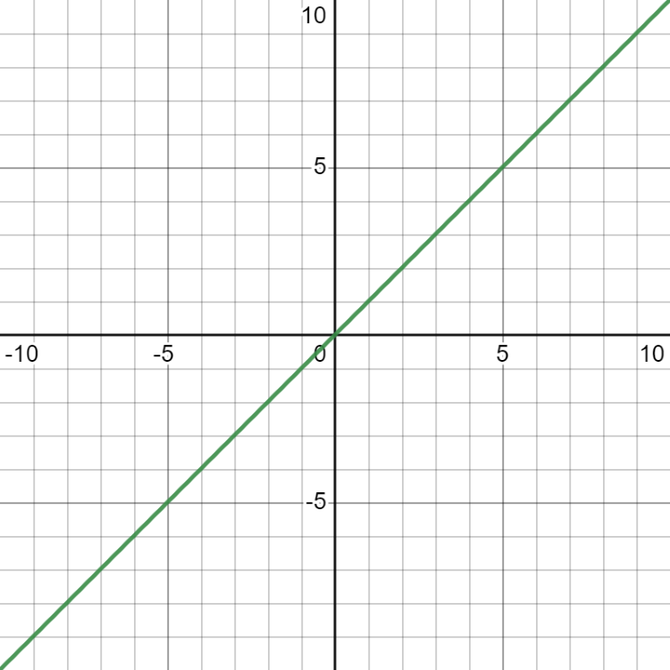
It imposes a complexity of O(N). It encompasses the same number of steps as that of the total number of elements to implement an operation on N elements.

Example: The below program takes Linear complexity.

Element is present at index 3

4. Quadratic Complexity: 

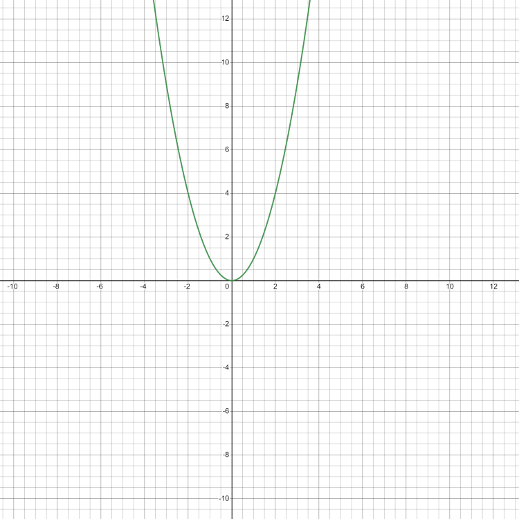
It imposes a complexity of O(n²). For N input data size, it undergoes the order of N² count of operations on N number of elements for solving a given problem.

Example: The below program takes quadratic complexity.

Yes

5. Factorial Complexity: 

It imposes a complexity of O(n!). For N input data size, it executes the order of N! steps on N elements to solve a given problem.

Example: The below program takes factorial complexity.

ABC
ACB
BAC
BCA
CBA
CAB

6. Exponential Complexity: 

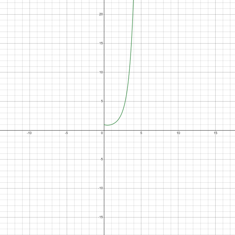
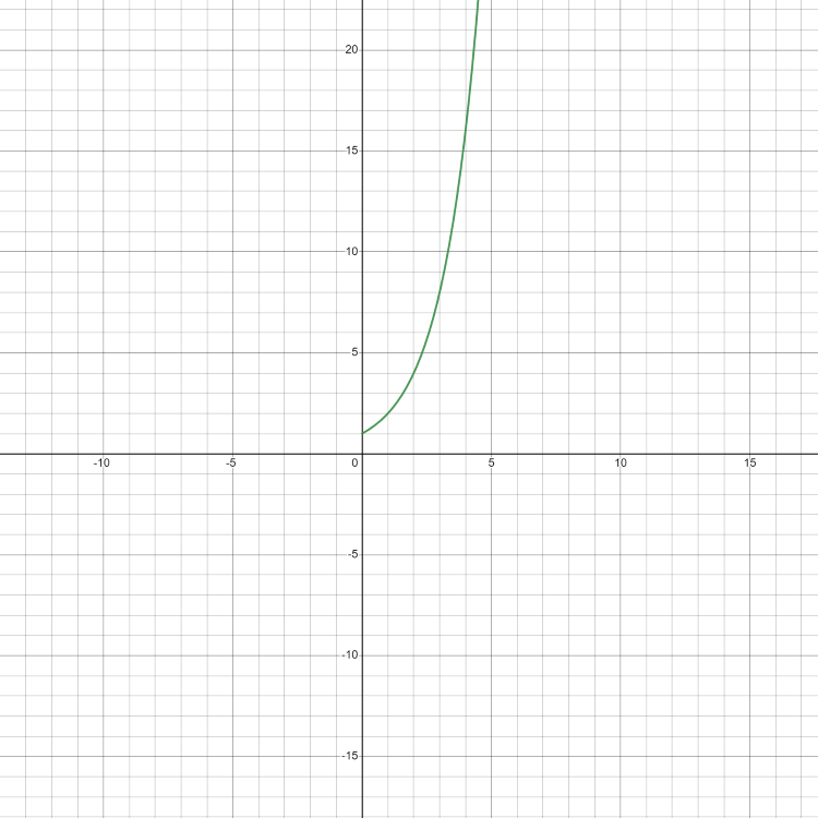
It imposes a complexity of O(2^N), O(N!), O(nk), …. For N elements, it will execute the order of the count of operations that is exponentially dependable on the input data size. 

Example: The below program takes exponential complexity.

Found a subset with given sum

Worst Case time complexity of different data structures for different operations

Complexity Analysis Of Popular Algorithms:

Practice some questions on Complexity Analysis:

• Practice Questions on Time Complexity Analysis
• Miscellaneous Problems of Time Complexity
• Sample Practice Problems on Complexity Analysis of Algorithm

Practice with giving  Quiz :

• Top MCQs on Complexity Analysis of Algorithms with Answers
• Top MCQs on NP-Complete Complexity with Answers
• Top MCQs on Complexity Analysis using Recurrence Relations with Answers

Conclusion:

Complexity analysis is a very important technique to analyze any problem. The interviewer often checks your ideas and coding skills by asking you to write a code giving restrictions on its time or space complexities. By solving more and more problems anyone can improve their logical thinking day by day. Even in coding contests optimized solutions are accepted. The naive approach can give TLE(Time limit exceed).