Chi-Square Test

The Chi-squared (χ²) test is a statistical method used to determine whether there is a significant association between two categorical variables or whether observed data fits an expected distribution. In categorical data analysis, the chi-square test compares observed frequencies with expected frequencies under a given hypothesis.

Chi-squared test, or χ² test, helps in determining whether these two variables are associated with each other.

This test is widely used in market research, healthcare, social sciences, and more to analyze categorical relationships.

For example, Entity 1: People’s favorite colors and Entity 2: Their preference for ice cream.

• Null Hypothesis (H₀): Favorite color and ice cream preference are independent (no relationship).
• Alternative Hypothesis (H₁): They are dependent (a relationship exists).

By comparing observed survey data with expected frequencies (if no relationship existed), the Chi-Square test calculates a test statistic (χ²). If this value is large enough, we reject H₀, concluding that color preference does influence ice cream choice and vice versa.

Formula For Chi-Square Test

Symbols are broken down as follows:

• O_i: Observed frequency
• E_i: Expected frequency

Categorical Variables

Categorical variables classify data into distinct, non-numeric groups (e.g., colors, fruit types).

Key Characteristics:

1. Distinct Groups: No overlap (e.g., hair color: blonde, brunette).
2. Non-Numerical: No arithmetic meaning (e.g., "apple" ≠ "orange" numerically).
3. Limited Options: Fixed categories (e.g., traffic lights: red, yellow, green).

Example: "Do you prefer tea, coffee, or juice?" → Categories: tea/coffee/juice.

Steps for Chi-Square Test

Steps and an illustration of an example of how sex influences which type of ice-cream a person will choose using a chi-square test are added below:

Step 1: Define Hypothesis

• Null Hypothesis (H₀): The variables are independent.
• Alternative Hypothesis (H₁): The variables are dependent.

Step 2: Gather and Organize Data

Gather Information about the Two Category Variables: Before performing a chi-square test, you should have on hand information about two categorical variables you wish to observe.

• You must collect details on people’s sex (male or female) and their best flavors (e.g., chocolate, vanilla, strawberry).

Once this information is collected, it can be inserted into a contingency table.

The hypothesis is that men prefer vanilla while women prefer chocolate. So we need to record how many have chosen vanilla among all male respondents versus the number who chose chocolate out of all female respondents.

Here's an example of what a contingency table might look like:

Step 3: Calculate Expected Frequencies

• Get Observed Frequency: In any specific cell, the expected frequency can be described as the number of occurrences that would be expected if the two variables were independent.
• Expected Frequency Calculation: This involves multiplying the sums of rows and columns in proportion, then dividing by the total number of observations in a table.

Observed frequency is the table given above.

• Male and chocolate:
• Male and Vanilla:
• Male and Strawberry:
• Female and chocolate:
• Female and Vanilla:
• Female and Strawberry:

Step 4: Perform Chi-Square Test

Use Chi-Square Formula:

Step 5: Determine Degrees of Freedom (df)

df = (number of rows - 1) × (number of columns - 1)

Step 6: Find p-value

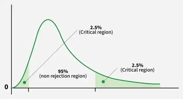
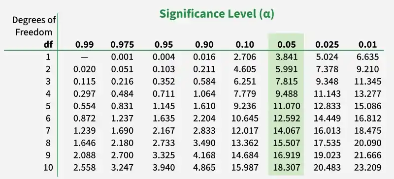
Compare the calculated χ² value with the critical value from the Chi-Square distribution table for the given degrees of freedom.

• If a predefined table is provided, use it
• Otherwise, we generally take the significance level as α = 0.05

Here, χ² = 4.86 with df=2:

Critical value at α=0.05 is 5.991.

Since 4.86 < 5.991, p > 0.05 

Step 7: Interpret Results

• If the p-value is less than a certain significance level (e.g., 0.05), then we reject the null hypothesis, which is commonly denoted by α. Thus, it means that category variables highly correlate with each other.
• When a p-value is above α, it implies that we cannot reject the null hypothesis; hence, there is insufficient evidence for establishing the relationship between these variables.

No significant evidence supports the claim that men prefer vanilla or women prefer chocolate (p>0.05).

Addressing Assumptions and Considerations

• Chi-square tests suppose that the observations are independent of one another; they are distinct.
• Each cell in the table should have a minimum of five values in it for better results. Otherwise, think about Fisher’s exact test as an alternative measure if a table cell has fewer than five numbers in it.
• Chi-square tests do not indicate a causal relationship, but they identify an association between variables.

Goodness-Of-Fit

A goodness-of-fit test checks if a hypothesized model matches observed data. For example, testing whether a die is fair.

Key Aspects:

1. Purpose: Check how well observed data fits expected data
2. Data Types: Categorical only
3. Applications: Compare observed vs. expected frequencies.
4. Benefits: Identifies model-data mismatch.

Applications of Chi-Square Test in Computer Science

A/B Testing & Feature Evaluation

• Compare user engagement (e.g., clicks, conversions) between two website versions (A vs. B).
• Chi-test is used to test if observed metrics (e.g., "Click" vs. "No Click") differ significantly between groups.
• Example: Observed: Version A: 120 clicks / 1,000 views; Version B: 150 clicks / 1,000 views. Chi-Square: Checks if the difference is statistically significant (not due to chance).

Machine Learning (Feature Selection)

• Identify categorical features correlated with target variables.
• Test if independence between features (e.g., "Browser Type" vs. "Purchase Decision") using the Chi-square test.
• Example: χ² p-value < 0.05 → "Browser Type" significantly affects purchases.

Database Query Optimization

• Assess if data is evenly distributed across partitions.
• Chi-square is used to test if actual row counts per partition match the expected uniform distribution.
• Example: Uneven distribution (χ² significance) suggests a poor sharding strategy.

Natural Language Processing (NLP)

• Evaluate word frequency distributions in texts.
• Compare observed word counts (e.g., "error" in logs) to the expected Poisson distribution.
• Example: Detects overused terms in spam emails (χ² highlights deviations from normal usage).

Solved Examples

Example 1: A study investigates the relationship between eye color (blue, brown, green) and hair color (blonde, brunette, Redhead). The following data is collected:

Step 1: Hypotheses

H₀: Eye color and hair color are independent
H₁: They are associated

Step 2: Expected Frequencies

Using

Blue: (40.91, 40.91, 18.18) {color: blonde,brunette,redhead }
Brown: (32.73, 32.73, 14.55)
Green: (16.36, 16.36, 7.27)

Step 3: Chi-Square Calculation

Step 4: Degrees of Freedom

df = (3 − 1)(3 − 1) = 4

Step 5: Decision

Critical value (α = 0.05, df = 4) = 9.488

Since 12.67 > 9.488 → Reject H₀

There is a significant association between eye color and hair color

Example 2: 100 flips of a coin are performed. The coin is fair, with an equal chance of heads and tails, according to the null hypothesis. 55 heads and 45 tails are the observed findings.

Step 1: Hypotheses

H₀: Coin is fair
H₁: Coin is not fair

Step 2: Expected Values

Heads = 50, Tails = 50

Step 3: Chi-Square Calculation

Step 4: Degrees of Freedom

df = 1

Step 5: Decision

Critical value (α = 0.05) = 3.84

Since 1 < 3.84 → Fail to reject H₀

The coin is likely fair

Related Articles:

• Chi-Square Test for Feature Selection
• Chi-square test in Machine Learning
• Application of Chi Square Test

Practice Problems

Q1. Market Research on Beverages

A company conducts a survey to determine whether there's a relationship between age groups and preferred beverages. The data collected is as follows:

Use a chi-square test to determine if there is an association between age groups and preferred beverages.

Q2. Student Performance

A teacher wants to find out if there is a relationship between study habits and grades. The data collected is as follows:

Perform a chi-square test to determine if study habits and grades are associated.

Q3. Gender and Major

A university wants to see if there is an association between gender and chosen major. The data collected is:

Conduct a chi-square test to examine if gender and chosen major are related.

Q4. Voting Preferences

A political analyst wants to know if there is a relationship between gender and voting preference. The data is:

Test the hypothesis that gender and voting preference are independent.