Exponential Smoothing is a statistical technique used to forecast future observations by assigning exponentially decreasing weights to past data points. It is applied in scenarios where data shows randomness, trends or seasonality.
Helps eliminate irregular spikes and dips caused by unpredictable events. Assigns higher importance to the most recent data without losing historical context. Works extremely well with continuously incoming observations. Smooth curves make it simpler to interpret upward or downward patterns. Requires minimal storage and performs fast calculations. Types of Exponential Smoothing 1. Simple or Single Exponential Smoothing Simple Smoothing is a forecasting method used for time series data that does not exhibit a trend or seasonality. It relies on univariate data and uses a single parameter called alpha ( ) or the smoothing factor.
determines how much weight is given to the current observation versus the past estimates. A smaller gives more importance to past predictions, while a larger emphasizes recent observations. The value of typically ranges from 0 to 1. The formula for simple smoothing is as follows:
Where:
: smoothed statistic (simple weighted average of current observation ) : previous smoothed statistic : smoothing factor of data; : time period 2. Double Exponential Smoothing Double Exponential Smoothing is a method used to forecast the trend of a time series that does not have seasonality. It's also called Holt’s Trend Model, second-order smoothing or Holt’s Linear Smoothing.
It accounts for trends in the data by introducing a trend component. It uses alpha to smooth the level of the series. It uses beta to smooth the trend or rate of change. It supports both additive and multiplicative trends. The formulas for Double exponential smoothing are as follows:
Where:
: best estimate of the trend at time : trend smoothing factor; 3. Holt-Winters’ Exponential Smoothing Triple exponential smoothing also known as Holt-Winters smoothing is a smoothing method used to predict time series data with both a trend and seasonal component. Gamma ( ) is used to control the effect of seasonal component.
The formulas for the triple exponential smoothing are as follows:
Where:
: smoothed statistic : previous smoothed statistic : smoothing factor of data : time period : best estimate of a trend at time t : trend smoothing factor : seasonal component at time : seasonal smoothing parameter Implementation Stepwise implementation of Exponential Smoothing:
1. Import Libraries Importing pandas and matplotlib library.
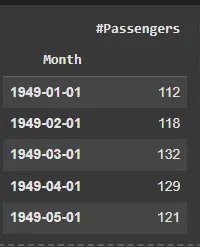
2. Load the Dataset Loading the dataset and inspect the first few rows.
pd.read_csv(): Reads the CSV file into a pandas DataFrame. parse_dates=['Month']: Converts the 'Month' column to a datetime format while loading the data. index_col='Month': Sets the 'Month' column as the index of the DataFrame. data.head(): Displays the first five rows of the dataset. Download lthe dataset from here
Output:
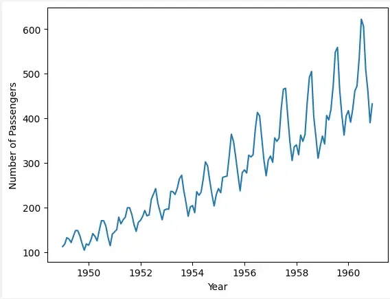
👁 dataset AirPassengers Dataset 3. Visualizing the Data Plotting the dataset and visualizing the number of passengers over time.
plt.plot(data): Plots the data. plt.xlabel('Year'): Labels the x-axis as "Year" to represent the time dimension of the dataset. plt.ylabel('Number of Passengers'): Labels the y-axis as "Number of Passengers" to indicate the metric being plotted. plt.show(): Displays the plot to visualize the data. Output:
👁 dataset_visual Visualizing the Data 4. Apply Single Exponential smoothing Applying simple exponential smoothing to the dataset using statsmodels library.
SimpleExpSmoothing(data): Initializes the Simple Exponential Smoothing model using the dataset data. model.fit(): Fits the model to the data, generating the smoothed values based on the provided dataset. Make Predictions
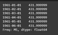
Forecasting the next 6 time periods using the fitted model.
model_single_fit.forecast(6) : Generates a forecast for the next 6 periods based on the fitted Simple Exponential Smoothing model. Output:
👁 single Single Exponential smoothing Visualize Single Exponential Smoothing
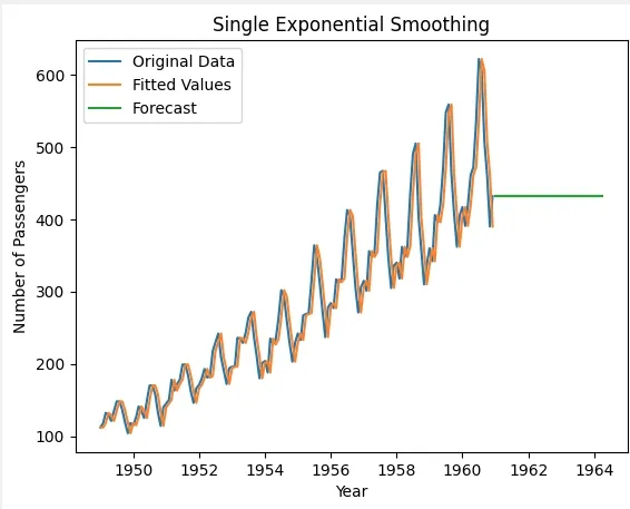
Visualizing the original data, fitted values and the forecasted values for the next 40 periods.
model_single_fit.forecast(40): Forecasts the next 40 periods using the fitted model. plt.plot(data, label='Original Data'): Plots the original dataset (number of passengers) with the label "Original Data". plt.plot(model_single_fit.fittedvalues, label='Fitted Values'): Plots the fitted values (smoothed data) from the model with the label "Fitted Values". plt.plot(forecast_single, label='Forecast'): Plots the forecasted values for the next 40 periods with the label "Forecast". plt.legend(): Displays the legend to differentiate between the original data, fitted values and forecast. plt.show(): Displays the plot for visualization. Output:
👁 single-graph Visualizing Single Exponential Smoothing 5. Apply Double Exponential Smoothing (Holt's Linear Trend) Applying Holt's linear trend method to the dataset for double exponential smoothing using statsmodels library.
Holt(data): Initializes the Holt's linear trend model using the dataset data. model_double.fit(): Fits the model to the data, capturing both level and trend in the series. Make Predictions
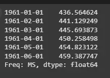
Forecasting the next 6 time periods using Holt's linear trend model.
Output:
👁 double Double Exponential Smoothing Visualizing Double Exponential Smoothing
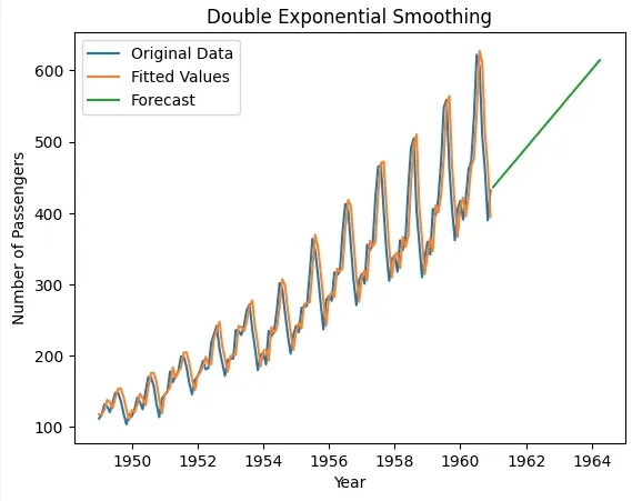
We will now visualize the original data, fitted values and forecasted values for the next 40 periods using Holt's method.
model_double_fit.forecast(40): Forecasts the next 40 periods using the fitted Holt's linear trend model. plt.plot(data, label='Original Data'): Plots the original dataset (number of passengers) with the label "Original Data". plt.plot(model_double_fit.fittedvalues, label='Fitted Values'): Plots the fitted values from the model with the label "Fitted Values". plt.plot(forecast_double, label='Forecast'): Plots the forecasted values for the next 40 periods with the label "Forecast". Output:
👁 double-graph Visualizing Double Exponential Smoothing 6. Apply Holt-Winter’s Seasonal Smoothing Applying triple exponential smoothing (Holt-Winters) to the dataset using statsmodels library.
ExponentialSmoothing(): Initializes the Exponential Smoothing model. seasonal_periods=12: Specifies a seasonal cycle of 12 periods like monthly data with yearly seasonality. trend='add': Specifies an additive trend component. seasonal='add': Specifies an additive seasonal component. model_triple.fit(): Fits the model to the data, incorporating the level, trend and seasonality. Making Predictions
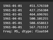
Forecasting the next 6 time periods using the fitted triple exponential smoothing model.
Output:
👁 triple Holt-Winter’s Seasonal Smoothing Visualize Triple Exponential Smoothing
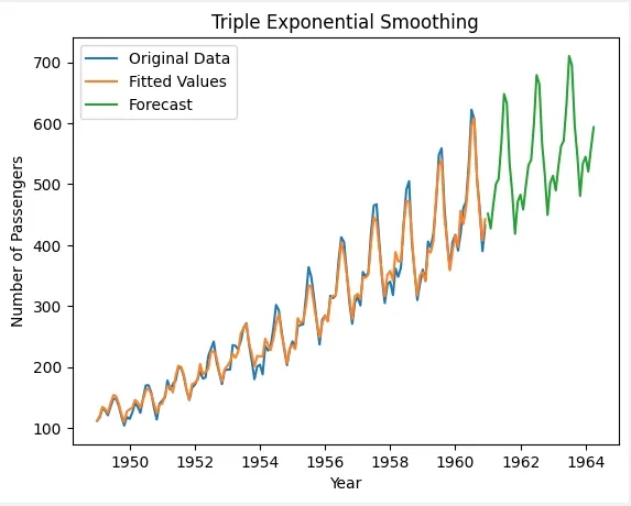
Visualize the original data, fitted values and forecasted values for the next 40 periods using triple exponential smoothing.
forecast_triple = model_triple_fit.forecast(40): Forecasts the next 40 periods using the fitted triple exponential smoothing model. plt.plot(data, label='Original Data'): Plots the original dataset (number of passengers) with the label "Original Data". plt.plot(model_triple_fit.fittedvalues, label='Fitted Values'): Plots the fitted values from the model with the label "Fitted Values". plt.plot(forecast_triple, label='Forecast'): Plots the forecasted values for the next 40 periods with the label "Forecast". Output:
👁 triple_graph Visualizing Triple Exponential Smoothing Choosing Exponential Smoothing Technique Guidelines for choosing an appropriate Exponential Smoothing technique are:
Method When to Use Description Example Simple Exponential Smoothing (SES) Time series with no trend or seasonality. Uses the most recent data point to forecast. Applied when data is stationary without clear trend or seasonality. Stock prices without a trend or season. Holt’s Linear Smoothing Time series with a trend but no seasonality. Extends SES to account for a linear trend. Forecasts data with consistent upward or downward movement. Sales data with steady growth. Holt-Winter’s Seasonal Smoothing Time series with both trend and seasonality. Adds a seasonal component to the trend, capturing both. Used for time series with repeating patterns and trends. Monthly temperature data or quarterly sales.
Advantages Easy to configure and requires fewer historical values compared to complex forecasting algorithms. Recent observations are prioritized, improving responsiveness to changing trends. Lightweight calculations make it suitable for real-time prediction environments and low-resource systems. Irregular fluctuations are minimized, producing clearer and more interpretable forecast lines. Different variants like Simple, Holt, Holt-Winters allow modeling of level, trend and seasonality. Disadvantages Abrupt spikes or drops in data can distort forecasts significantly. Incorrect selection of smoothing factors may lead to unstable or lagging predictions. Forecast quality decreases as the prediction horizon extends further into the future. Models may react excessively to random noise when smoothing values are high. 