How to perform faster convolutions using Fast Fourier Transform(FFT) in Python?

Convolution is one of the most important mathematical operations used in signal processing. This simple mathematical operation pops up in many scientific and industrial applications, from its use in a billion-layer large CNN to simple image denoising. Convolution can be both analog and discrete in nature, but because of modern-day computers' digital nature, discrete convolution is the one that we see all around!

The discrete convolution of two 1 dimensional vectors and ,  is defined as

As it requires the multiplication of two vectors, the time complexity of discrete convolution using multiplication(assuming vectors of length ) is . Here's where Fast Fourier transform(FFT) comes in. Using FFT, we can reduce this complexity from  to !

The intuition behind using FFT for convolution

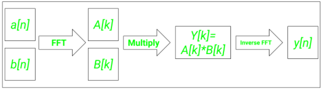
One of the most fundamental signal processing results states that convolution in the time domain is equivalent to multiplication in the frequency domain. For performing convolution, we can convert both the signals to their frequency domain representations and then take the inverse Fourier to transform of the Hadamard product (or dot product) to obtain the convoluted answer. The workflow can be summarized in the following way

Installation:

For this article's purposes, we'll be using some inbuilt functions from the Python libraries numpy and scipy. You can use the pip package manager to install them.

pip install scipy numpy

FFT convolution in Python

For computing convolution using FFT, we'll use the fftconvolve() function in scipy.signal library in Python.

Syntax: scipy.signal.fftconvolve(a, b, mode='full')

Parameters:

• a: 1st input vector
• b: 2nd input vector
• mode: Helps specify the size and type of convolution output
  • 'full': The function will return the full convolution output
  • 'same': The function will return an output with dimensions same as the vector 'a' but centered at the centre of the output from the 'full'  mode
  • 'valid': The function will return those values only which didn't rely on zero-padding to be computed

Below is the implementation:

Output

The convoluted sequence is [ 4. 13. 28. 27. 18.]

Performance comparison of FFT convolution with normal discrete convolution

• For computing the normal linear convolution of two vectors, we'll use the np.convolve function.
• The %timeit magic function of Jupyter notebooks was used to calculate the total time required by each of the 2 functions for the given vectors.

Below is the implementation:

Output:

Time required for normal discrete convolution:
1.1 s ± 245 ms per loop (mean ± std. dev. of 7 runs, 1 loop each)
Time required for FFT convolution:
17.3 ms ± 8.19 ms per loop (mean ± std. dev. of 7 runs, 10 loops each)

You can see that the output generated by FFT convolution is 1000 times faster than the output produced by normal discrete convolution!