Cubic spline Interpolation

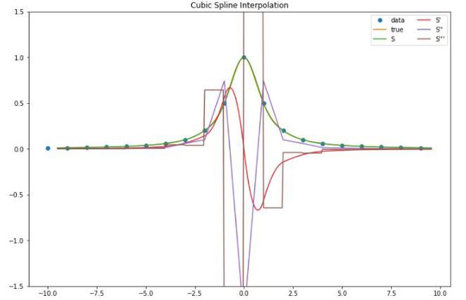
Cubic Spline Interpolation is a method used to draw a smooth curve through a set of given data points. Instead of connecting the points with straight lines or a single curve, it fits a series of cubic polynomials between each pair of points. These polynomials join smoothly, making the curve look natural and continuous. This technique is especially useful when we want smooth and accurate results from scattered data.

What is Interpolation

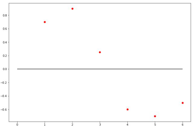
We estimate f(x) for arbitrary x, by drawing a smooth curve through the x_i. If the desired x is between the largest and smallest of the x_i then it is called interpolation, otherwise, it is called Extrapolation.

Different Types of Interpolation

Linear Interpolation

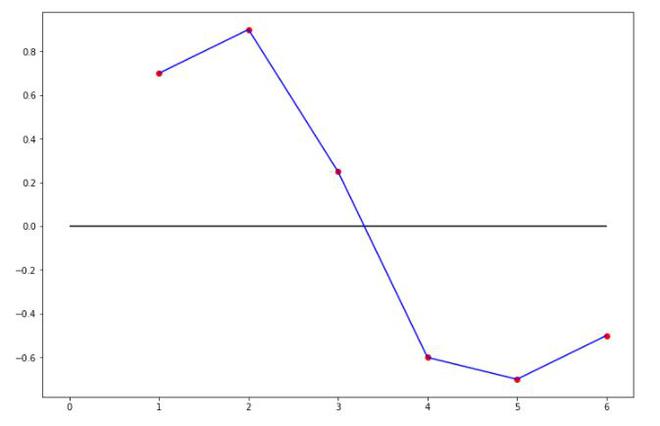
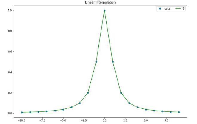
Linear Interpolation is a way of curve fitting the points by using linear polynomial such as the equation of the line. This is just similar to joining points by drawing a line b/w the two points in the dataset.

Polynomial Interpolation

Polynomial Interpolation is the way of fitting the curve by creating a higher degree polynomial to join those points.

Spline Interpolation

Spline interpolation similar to the Polynomial interpolation x' uses low-degree polynomials in each of the intervals and chooses the polynomial pieces such that they fit smoothly together. The resulting function is called a spline.

Cubic Spline Interpolation

Given data points , the goal is to fit piecewise cubic polynomials over each interval , such that:

Let and define second derivatives at the knots as . From Taylor approximation and spline properties:

Which leads to the spline equation:

Where:

This forms a tridiagonal matrix system to solve for M₀, M₁, ..., M_n​. Once second derivatives M_i​ are known, the spline on each interval is:

Where constants and depend on and ​.

Cubic spline Interpolation Implementation in Python

We will be using the Scipy to perform the linear spline interpolation. We will be using Cubic Spline and interp1d function of scipy to perform interpolation of function

Output:

Advantages of Cubic Spline Interpolation

• Smooth and Continuous Curves: Produces a smooth curve with continuous first and second derivatives, ensuring natural transitions between points.
• Accurate Approximation: Provides a better fit than linear or quadratic interpolation, especially when modeling curved data.
• Local Control: Each spline segment only depends on a few data points, so changes in one part don't drastically affect the entire curve.

Challenges of Cubic Spline Interpolation

• Computational Complexity: Requires solving a system of equations, which may be computationally expensive for large datasets.
• Boundary Conditions Sensitivity: Different choices of boundary conditions (natural, clamped, etc.) can affect the shape of the spline.
• Overfitting Risk: If data contains noise, the spline may fit the noise too closely, reducing generalization accuracy.

Applications of Cubic Spline Interpolation

1. Computer Graphics and Animation: Used for smooth curve modeling and motion paths in design and animation.
2. Engineering and CAD: Helps in designing smooth mechanical components, surfaces and motion trajectories.
3. Scientific and Statistical Data Fitting: Ideal for creating smooth curves from experimental or observed data in physics, biology, or economics.