Dilated Convolution

Prerequisite: Convolutional Neural Networks

Dilated Convolution: It is a technique that expands the kernel (input) by inserting holes between its consecutive elements. In simpler terms, it is the same as convolution but it involves pixel skipping, so as to cover a larger area of the input. 

Dilated convolution, also known as atrous convolution, is a type of convolution operation used in convolutional neural networks (CNNs) that enables the network to have a larger receptive field without increasing the number of parameters.

In a regular convolution operation, a filter of a fixed size slides over the input feature map, and the values in the filter are multiplied with the corresponding values in the input feature map to produce a single output value. The receptive field of a neuron in the output feature map is defined as the area in the input feature map that the filter can "see". The size of the receptive field is determined by the size of the filter and the stride of the convolution.

In contrast, in a dilated convolution operation, the filter is "dilated" by inserting gaps between the filter values. The dilation rate determines the size of the gaps, and it is a hyperparameter that can be adjusted. When the dilation rate is 1, the dilated convolution reduces to a regular convolution.

The dilation rate effectively increases the receptive field of the filter without increasing the number of parameters, because the filter is still the same size, but with gaps between the values. This can be useful in situations where a larger receptive field is needed, but increasing the size of the filter would lead to an increase in the number of parameters and computational complexity.

Dilated convolutions have been used successfully in various applications, such as semantic segmentation, where a larger context is needed to classify each pixel, and audio processing, where the network needs to learn patterns with longer time dependencies.

Some advantages of dilated convolutions are:

1. Increased receptive field without increasing parameters
2. Can capture features at multiple scales
3. Reduced spatial resolution loss compared to regular convolutions with larger filters

Some disadvantages of dilated convolutions are:

1. Reduced spatial resolution in the output feature map compared to the input feature map
2. Increased computational cost compared to regular convolutions with the same filter size and stride

References:

1. Holschneider, M., Kronland-Martinet, R., Morlet, J., & Tchamitchian, P. (1989). A real-time algorithm for signal analysis with the help of the wavelet transform. In Wavelets (pp. 286-297). Springer.
2. Yu, F., & Koltun, V. (2016). Multi-scale context aggregation by dilated convolutions. arXiv preprint arXiv:1511.07122.
   Chen, L. C., Papandreou, G., Kokkinos, I., Murphy, K., & Yuille, A. L. (2018). Deeplab: Semantic image segmentation with deep convolutional nets, atrous convolution, and fully connected crfs. IEEE transactions on pattern analysis and machine intelligence, 40(4), 834-848.

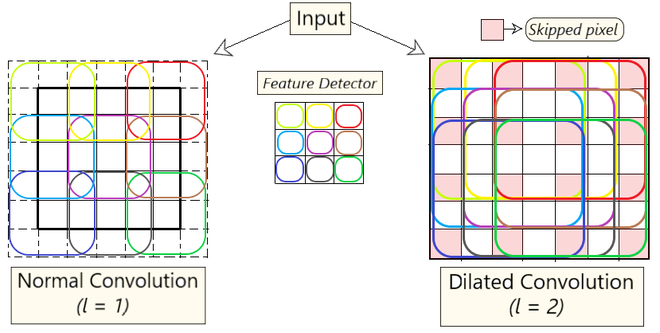
An additional parameter l (dilation factor) tells how much the input is expanded. In other words, based on the value of this parameter, (l-1) pixels are skipped in the kernel. Fig 1 depicts the difference between normal vs dilated convolution. In essence, normal convolution is just a 1-dilated convolution.

👁 Image

Intuition: 

Dilated convolution helps expand the area of the input image covered without pooling. The objective is to cover more information from the output obtained with every convolution operation. This method offers a wider field of view at the same computational cost. We determine the value of the dilation factor (l) by seeing how much information is obtained with each convolution on varying values of l.  

By using this method, we are able to obtain more information without increasing the number of kernel parameters. In Fig 1, the image on the left depicts dilated convolution. On keeping the value of l = 2, we skip 1 pixel (l - 1 pixel) while mapping the filter onto the input, thus covering more information in each step. 

Formula Involved: 

where,
F(s) = Input 
k(t) = Applied Filter
*l = l-dilated convolution
(F*lk)(p) = Output

Advantages of Dilated Convolution:   

Using this method rather than normal convolution is better as: 

1. Larger receptive field (i.e. no loss of coverage)
2. Computationally efficient (as it provides a larger coverage on the same computation cost)
3. Lesser Memory consumption (as it skips the pooling step) implementation
4. No loss of resolution of the output image (as we dilate instead of performing pooling)
5. Structure of this convolution helps in maintaining the order of the data. 

Code Implementation: 

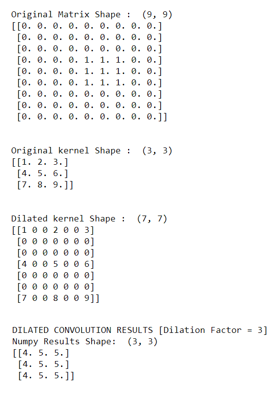
 Output 

The following output is obtained from the above code.  

👁 Image

 

The output obtained is for a dilation factor of 3. For more experimentation, you can initialize the dilated_kernel with different values of the Dilation factor and observe the changes in the output obtained.