Dirichlet Distribution

The Dirichlet distribution is a multivariate extension of the Beta distribution and is extensively applied in Bayesian statistics and machine learning. It is used to model categorical data, proportions, and probabilities and acts as a conjugate prior for multinomial distributions. Some of its important properties are its use in Bayesian inference and parameter estimation simplicity.

The Dirichlet distribution is a multivariate continuous family of probability distributions parameterized by a vector α (alpha), with each αᵢ > 0. It is a probability simplex, i.e., the components of a Dirichlet-distributed random variable add up to 1.

Mathematically

if X = (X₁, X₂,., Xₖ) is Dirichlet distributed with parameter vector α = (α₁, α₂,., αₖ), then its probability density function (PDF) is:

where X₁, X₂, ..., Xₖ are non-negative and satisfy:

The normalization constant B(α) (also called the multivariate Beta function) ensures that the probability density integrates to 1 and is defined as:

​where Γ(αᵢ) is the Gamma function, which generalizes the factorial function.

Properties of Dirichlet Distribution

1. Expectation (Mean)

The mean of each component Xᵢ in a Dirichlet-distributed random variable is given by:

​This shows that each expected proportion depends on its corresponding parameter αᵢ relative to the sum of all α parameters.

2. Variance and Covariance

The variance of each component is:

The covariance between two components Xᵢ and Xⱼ (for i ≠ j) is:

This negative covariance indicates that an increase in one component leads to a decrease in others due to the constraint that their sum is 1.

3. Relationship with Beta Distribution

The Dirichlet distribution is a generalization of the Beta distribution. Specifically, for k = 2, the Dirichlet distribution reduces to a Beta distribution:

Practical Example

We are a market analyst estimating the proportions of customer preferences for three brands. We believe that the prior probabilities for the market share are approximately:

• Brand A: 50%
• Brand B: 30%
• Brand C: 20%

These prior beliefs can be modeled using a Dirichlet distribution with the parameter vector:

α = ( 5, 3, 2)

Here:

• 𝛼₁ = 5 corresponds to Brand A
• 𝛼₂ = 3 corresponds to Brand B
• 𝛼₃ = 2 corresponds to Brand C

The values of 𝛼 reflect the concentration of beliefs:

• Larger values → more confident priors
• Smaller values → more uncertain priors

1. Dirichlet Distribution PDF

The probability density function (PDF) for the three-brand scenario is given by:

Where:

The normalization constant is the multivariate Beta function:

Using the Gamma function values:

2. Sampling from the Distribution

If we sample from this Dirichlet distribution, we get probability vectors representing possible market share proportions.

For example, some sampled vectors could be:

Brand A dominates

(0.48, 0.32, 0.20) Brand B has increased slightly

Even split according to prior belief

These vectors indicate the probabilistic nature of the Dirichlet distribution, where the proportions vary but still sum to 1.

Practical Implementation in Python

The scipy.stats library provides functions to work with the Dirichlet distribution.

Sampling from a Dirichlet Distribution

Output

[[0.27190357 0.0975921 0.63050434]
 [0.05886627 0.42894514 0.51218859]
 [0.10245169 0.39020273 0.50734557]
 [0.17880239 0.21161496 0.60958265]
 [0.06295282 0.33473457 0.60231261]]

Plotting a 2D Dirichlet Distribution

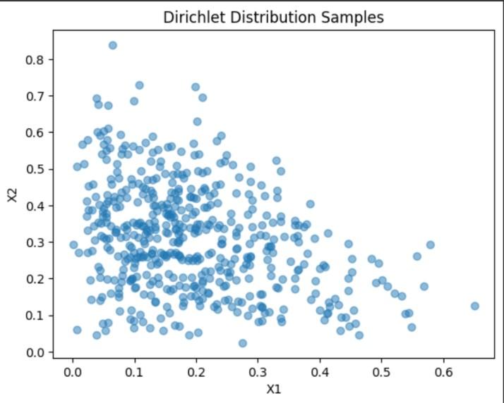
For visualization, we can plot the probability simplex:

This provides insight into how probability distributions are generated from the Dirichlet prior.

Output:

Parameter Estimation for Dirichlet Distribution

Having a sample of observed probability vectors X₁, X₂,., Xₙ, we would like to estimate the Dirichlet distribution parameters α.

Method of Moments Estimation

The method of moments estimates α based on sample means:

This approach is simple but less accurate than maximum likelihood estimation.

Maximum Likelihood Estimation (MLE)

The MLE approach finds α by maximizing the likelihood function:

However, this requires numerical optimization techniques, such as Newton’s method or the fixed-point iteration method, because there is no closed-form solution.

Applications of Dirichlet Distribution

• Bayesian Inference: Used as a conjugate prior for the multinomial distribution, ensuring that both prior and posterior distributions remain Dirichlet in Bayesian modeling.
• Topic Modeling (LDA): Applied in Latent Dirichlet Allocation (LDA) to model topic distributions in documents and word distributions within topics, making it essential in natural language processing.
• Mixture Models & Clustering: Utilized in Dirichlet Process Mixture Models (DPMMs), extending Gaussian Mixture Models (GMMs) to handle an unknown number of clusters.
• Probability Estimation: Helps model uncertainty over categorical probabilities in applications like genetics, polls, and marketing