 |
VOOZH | about |
|
VOOZH | about |
From the perspective of Industrial Companies that run with huge employees, employee attrition is a significant concern for many organizations as it affects productivity and financial health. Predicting which employees are likely to leave can help companies implement strategies to retain and hire valuable talent. In this article, we will explore how to predict employee attrition using the R Programming Language.
The main objectives of this project are:
This data set is collected from the IBM Human Resources department. The dataset contains 1470 observations and 35 variables. Within 35 variables “Attrition” is the dependent variable in the dataset.
Dataset Link: Employee Attrition
The dataset was collected through HR records and employee surveys. Key features inside the dataset includes:
We use the readr and the dplyr packages in R for loading and inspecting the dataset.
Output:
 Age Attrition BusinessTravel DailyRate Department DistanceFromHome
1 41 Yes Travel_Rarely 1102 Sales 1
2 49 No Travel_Frequently 279 Research & Development 8
3 37 Yes Travel_Rarely 1373 Research & Development 2
4 33 No Travel_Frequently 1392 Research & Development 3
5 27 No Travel_Rarely 591 Research & Development 2
6 32 No Travel_Frequently 1005 Research & Development 2
 Education EducationField EmployeeCount EmployeeNumber EnvironmentSatisfaction
1 2 Life Sciences 1 1 2
2 1 Life Sciences 1 2 3
3 2 Other 1 4 4
4 4 Life Sciences 1 5 4
5 1 Medical 1 7 1
6 2 Life Sciences 1 8 4
 Gender HourlyRate JobInvolvement JobLevel JobRole JobSatisfaction
1 Female 94 3 2 Sales Executive 4
2 Male 61 2 2 Research Scientist 2
3 Male 92 2 1 Laboratory Technician 3
4 Female 56 3 1 Research Scientist 3
5 Male 40 3 1 Laboratory Technician 2
6 Male 79 3 1 Laboratory Technician 4
 MaritalStatus MonthlyIncome MonthlyRate NumCompaniesWorked Over18 OverTime
1 Single 5993 19479 8 Y Yes
2 Married 5130 24907 1 Y No
3 Single 2090 2396 6 Y Yes
4 Married 2909 23159 1 Y Yes
5 Married 3468 16632 9 Y No
6 Single 3068 11864 0 Y No
 PercentSalaryHike PerformanceRating RelationshipSatisfaction StandardHours
1 11 3 1 80
2 23 4 4 80
3 15 3 2 80
4 11 3 3 80
5 12 3 4 80
6 13 3 3 80
 StockOptionLevel TotalWorkingYears TrainingTimesLastYear WorkLifeBalance
1 0 8 0 1
2 1 10 3 3
3 0 7 3 3
4 0 8 3 3
5 1 6 3 3
6 0 8 2 2
 YearsAtCompany YearsInCurrentRole YearsSinceLastPromotion YearsWithCurrManager
1 6 4 0 5
2 10 7 1 7
3 0 0 0 0
4 8 7 3 0
5 2 2 2 2
6 7 7 3 6
We have to check if there are any missing values in the dataset. In case of any missing values found, the function below returns 1 in the output.
Output:
[1] 0Visualizing the data before feeding it into a model is a most important step in making the target audience understand you analysis and prediction and upon what base does your prediction stand by.
Visualizing the data before feeding it into a model is crucial for several reasons:
Output:
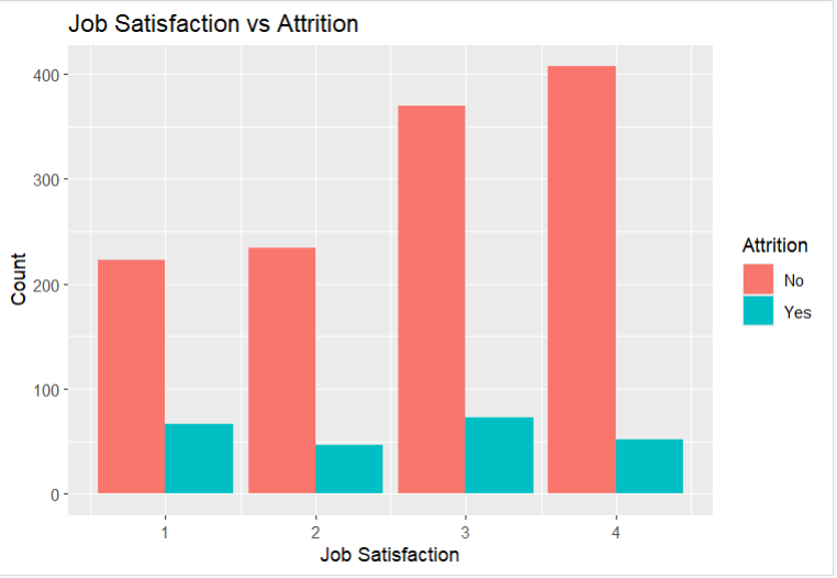
Now we will Plot the relationship between job satisfaction and attrition.
Output:
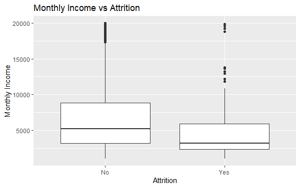
Now we will Plot the relationship between monthly income and attrition.
Output:
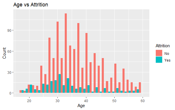
Now we will Plot the relationship between age and attrition.
Output:
With the help of the Training data set we will build up our model and test its accuracy using the Testing Data set.
We have successfully split the whole data set into two parts. Now we have 1025 Training data & 445 Testing data.
Now we will build model using Random Forest that constructs multiple decision trees during training and outputs the mode of the classes (classification) or mean prediction (regression) of the individual trees. It improves predictive accuracy and controls overfitting.
Output:
Call:
 randomForest(formula = Attrition ~ ., data = trainData, importance = TRUE)
 Type of random forest: classification
 Number of trees: 500
No. of variables tried at each split: 5

 OOB estimate of error rate: 13.88%
Confusion matrix:
 No Yes class.error
No 857 7 0.008101852
Yes 136 30 0.819277108

Confusion Matrix and Statistics

 Reference
Prediction No Yes
 No 366 59
 Yes 3 12

 Accuracy : 0.8591
 95% CI : (0.823, 0.8902)
 No Information Rate : 0.8386
 P-Value [Acc > NIR] : 0.1345

 Kappa : 0.2361

 Mcnemar's Test P-Value : 2.848e-12

 Sensitivity : 0.9919
 Specificity : 0.1690
 Pos Pred Value : 0.8612
 Neg Pred Value : 0.8000
 Prevalence : 0.8386
 Detection Rate : 0.8318
 Detection Prevalence : 0.9659
 Balanced Accuracy : 0.5804

 'Positive' Class : No
OverTime and MonthlyIncome are the most important factors influencing attrition.
Based on the above analysis, prediction and findings, Logistic Regression and Random Forest models provide valuable insights into the factors influencing employee attrition.Predicting employee attrition using machine learning models in R provides a valuable insights into the factors driving turnover(Employee Attrition). By understanding these factors, organizations can implement targeted strategies to retain their top talent, thereby enhancing productivity and reducing the costs associated with employee turnover.