Fitting Logarithmic Curve in a Dataset in R

Fitting a logarithmic curve to a dataset in R involves finding parameters that best describe the logarithmic relationship between variables. Logarithmic curves are often used to model situations where the growth rate of a variable decreases over time or with increasing values of another variable. Here's a step-by-step guide on how to fit a logarithmic curve to a dataset using R:

Understanding Logarithmic Curves

A logarithmic curve typically represents a relationship where one variable changes logarithmically to another variable.

Here's a step-by-step guide on how to fit a logarithmic curve to a dataset using R Programming Language:

Step 1: Load Necessary Libraries

First, load the necessary libraries. We'll use ggplot2 for plotting and nls() for fitting the nonlinear least squares regression model.

Step 2: Generate Example Data

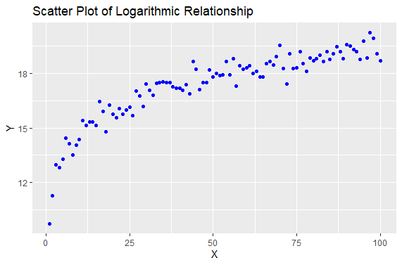
Create an example dataset. For demonstration purposes, we'll create a dataset where x and y variables exhibit a logarithmic relationship.

Step 3: Plot the Data

Visualize the data using a scatter plot to understand the relationship between x and y.

Output:

Step 4: Fit the Logarithmic Curve

Fit a logarithmic curve to the data using nls() (nonlinear least squares). We'll use a logarithmic function of the form y=a+b⋅log⁡(x) where a and b are parameters to be estimated.

Output:

Formula: y ~ a + b * log(x)

Parameters:
 Estimate Std. Error t value Pr(>|t|) 
a 9.97994 0.18631 53.57 <2e-16 ***
b 2.01794 0.04965 40.65 <2e-16 ***
---
Signif. codes: 0 ‘***’ 0.001 ‘**’ 0.01 ‘*’ 0.05 ‘.’ 0.1 ‘ ’ 1

Residual standard error: 0.4584 on 98 degrees of freedom

Number of iterations to convergence: 1 
Achieved convergence tolerance: 1.154e-08

• The fitted model y=9.97994+2.01794⋅log⁡(x) suggests a strong logarithmic relationship between x and y.
• Both coefficients are highly significant (p < 2e-16), indicating that they are meaningful predictors of y.
• The residual standard error is 0.4584, indicating a reasonably good fit to the data.
• The model converged quickly with a high degree of precision.

By fitting this logarithmic model, you can interpret the relationship between x and y in a meaningful way, understanding how changes in x (in the logarithmic scale) are associated with changes in y.

Step 5: Visualize the Fitted Curve

Plot the fitted logarithmic curve along with the original data points to visualize how well the model fits the data.

Output:

We plot the original data points and overlay the fitted logarithmic curve to assess how well the model captures the data's logarithmic pattern.

Conclusion

Fitting a logarithmic curve to a dataset in R involves using nonlinear regression techniques. By following the steps outlined in this guide, you can effectively model and visualize logarithmic relationships between variables in your data. Adjust the model and plotting parameters based on your specific dataset and analytical requirements.