Heteroscedasticity refers to a violation of one of the key assumptions of linear regression constant variance of the error term. In an ideal regression model, residuals should be randomly scattered with equal spread (homoscedasticity). However, when the variance of residuals increases or decreases with the fitted values or predictor variables, the model becomes heteroscedastic. This affects the reliability of statistical inference, leading to inefficient estimates and invalid hypothesis tests.
Key Assumptions of Linear Regression
Errors have zero mean.
Errors have constant variance (homoscedasticity).
Errors are independent (no autocorrelation).
Errors follow a normal distribution.
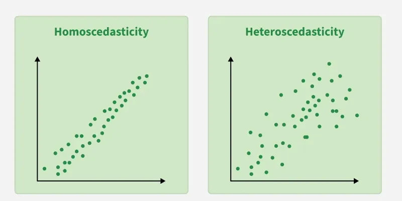
Homoscedasticity vs Heteroscedasticity
Lets compare Homoscedasticity and Heteroscedasticity,
Yes – may require WLS, transformation or robust errors
Reasons for Heteroscedasticity
Large variation between smallest and largest values (presence of outliers).
Incorrect model specification, such as missing variables or wrong functional form.
Mixing observations from different measurement scales.
Using incorrect transformations while preprocessing.
Skewed distribution of one or more independent variables.
Natural growth processes (e.g., income vs expenditure).
Effects
OLS estimators remain unbiased, but they are no longer efficient (not minimum variance).
Violates the BLUE (Best Linear Unbiased Estimator) property.
Standard errors become incorrect → t-tests and F-tests become unreliable.
Confidence intervals may become too wide or too narrow.
Model interpretations become misleading.
Identifying Heteroscedasticity
1. Graphical Method (Residual Plots)
Residual diagnostics are often the quickest way to spot heteroscedasticity. The most common plot is Residuals vs Fitted Values, where the residuals should appear randomly scattered. A model has heteroscedasticity when the plot shows:
Funnel or cone shapes: the spread of residuals increases or decreases as fitted values grow.
Systematic patterns: curved bands, clusters or waves instead of uniform scattering.
Non-constant scatter across ranges of the predictor variables.
Residual variation linked to specific groups in the data, indicating different variance levels across segments.
These visual cues indicate that the error variance is not constant and violates regression assumptions.
2. Statistical Tests for Heteroscedasticity
Graphical checks are intuitive, but statistical tests provide formal evidence.
1. Breusch–Pagan (BP) Test
Evaluates whether residual variance is related to the predictors.
The squared residuals are regressed on the independent variables.
A significant test statistic indicates that error variance changes systematically with predictors.
2. White Test
A more general test that does not assume any specific pattern of heteroscedasticity. Uses an auxiliary regression where squared residuals are regressed on:
original predictors,
their squares,
and their cross-products.
Detects both linear and nonlinear forms of heteroscedasticity. These tests help confirm heteroscedasticity even when visual patterns are subtle or ambiguous.
Corrections
Respecify the model (add missing variables, remove unnecessary ones).
