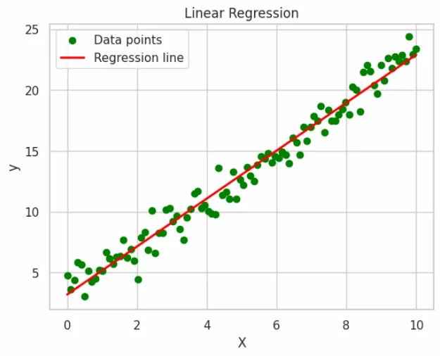
Linear Regression is a widely used supervised learning algorithm that assumes a linear relationship exists between input X and output Y. It computes parameters that minimize the cost function during the training phase. The objective is to find that minimizes the following cost function:
Where:
is the feature vector of the training example.
is the corresponding output value of the training example.
is the vector of parameters (weights) that we want to optimize.
👁 Linear-regression Visual Representation of Linear Regression on Linear Distribution
Prediction: For a given query point , the output is predicted as,
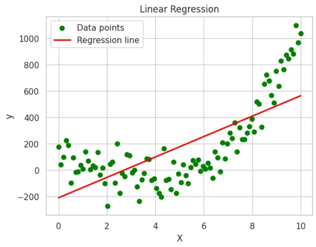
However when the relationship between X and Y is non-linear, the standard linear regression model may not be effective. In such cases, Locally Weighted Linear Regression (LWLR) is used.
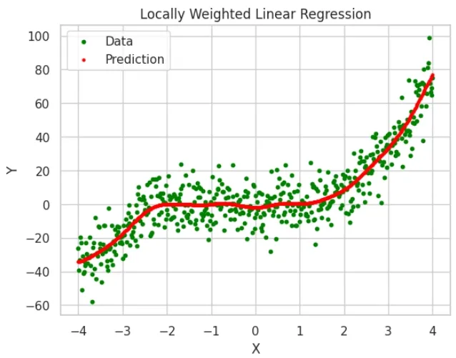
Locally Weighted Linear Regression (LWLR) is a flexible method that adjusts the model to focus on the data points closest to each query point. Instead of creating one overall model like traditional linear regression, it creates a separate model for each prediction, using only the nearby data. This makes it useful when data behaves differently in different parts. The cost function is adjusted as follows:
Where:
is the weight associated with the data point.
The weight is calculated using a Gaussian kernel function and it decreases as the distance between and increases.
The weight for each training point is computed using the following formula:
Where:
is the bandwidth parameter that controls the rate at which the weight decreases as the distance from increases.
When is small, the weight is close to 1.
When is large, the weight becomes very small, approaching 0.
Example: Consider a query point x=5.0x = 5.0x=5.0 and two training points:
= 4.9
= 3.0
Using the weight formula with , the weights are computed as:
As we can see, the weight for the closer point is much larger than the weight for the farther point . Thus, the contribution of to the cost function is far greater than that of , ensuring that the model fits the data locally around the query point.
Key Features of LWLR
Non-parametric: No global model, computes unique parameters for each query point.
Local adaptation: Focuses on nearby data points for predictions.
Weighted points: Closer points have more influence, distant points have less.
Handles non-linearity: Great for complex, non-linear data relationships.
No global parameters: Uses local fits instead of a single, global model.
Steps Involved in Locally Weighted Linear Regression:
1. Compute Weights: For each data point , compute the weight using the distance from the query point . The weight is computed using the gaussian kernel function:
Where:
is bandwidth parameter that controls how quickly the weight decreases with distance.
is a training example and is the query point (the point for which we are making the prediction).
2. Formulate the Weighted Cost Function: Once the weights have been computed for all training examples, the weighted cost function is formulated as:
Where:
represents the parameters (or weights) of the model that we need to optimize.
is the feature vector of the training example.
is the output value of the training example.
is the total number of training examples.
3. Solve for Parameters using Weighted Least Squares: The optimal parameter vector is found by minimizing the weighted cost function using the closed-form solution:
Where:
X is the matrix of all feature vectors (training data).
W is the diagonal matrix of weights where each diagonal element corresponds to the weight of the training point.
y is the vector of output values.
4. Prediction: For a given query point x, the predicted output is:
This is a linear combination of the input features of the query point weighted by the parameters obtained from the local regression model.
Application
Non-linear Regression: Models complex, non-linear relationships in data.
Time Series Forecasting: Forecasts future values by focusing on recent data like stock prices, energy demand, etc.
Anomaly Detection: Detects outliers by comparing local predictions with actual values like fraud detection.
Robotics: Used in adaptive control and path planning for robots like self-driving cars.
Medical Data Analysis: Predicts disease progression based on non-linear relationships in patient data like cancer progression.
Advantages of LWLR
Flexibility: Can model non-linear relationships by focusing on local data points.
Adaptivity: Adjusts to local patterns, making it suitable for dynamic or non-stationary data.
Precision: Provides better predictions for data with varying characteristics across different regions.
No Global Model: Creates a new model for each prediction, making it highly customized to the query point.
Simple and Intuitive: Easy to implement and understand compared to more complex models.
Limitations
Computationally Expensive: Can be slow for large datasets due to the need to compute weights and solve for parameters for each query point.
Sensitive to Bandwidth (): The performance heavily depends on the choice of the bandwidth parameter, requiring careful tuning.
No Global Model: Lacks a single, unified model which can make it harder to interpret or generalize.
Overfitting Risk: In areas with sparse data, the model may overfit to noise or anomalies.
Limited Scalability: May not perform well on very large datasets without optimization techniques.
