Monte Carlo Tree Search (MCTS) is a method used for problems with very large decision spaces, such as game Go, which has around 10¹⁷⁰ possible states. It builds a search tree step-by-step using random simulations to choose better moves.

• Avoids exploring every possible move.
• Balances trying new moves (exploration) and using good known moves (exploitation).
• Uses statistical sampling to guide decisions.
• Works well when the search space is too large to evaluate fully.

The Four-Phase Algorithm

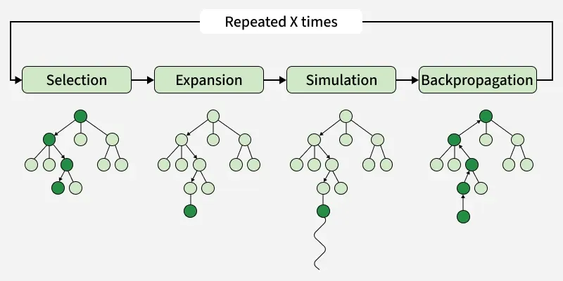
1. Selection : Starting at the root node, MCTS moves down the tree using a selection rule. The most common rule is UCT (Upper Confidence Bounds for Trees), which balances:

• Exploitation: choosing moves with higher average reward
• Exploration: trying moves with less information

2. Expansion : When the selection phase reaches a leaf node that isn't terminal, the algorithm expands the tree by adding one or more child nodes representing possible actions from that state.

3. Simulation Phase: From the newly added node, a random playout is performed until reaching a terminal state. During this phase, moves are chosen randomly or using simple heuristics, making the simulation computationally inexpensive.

4. Backpropagation Phase: The result of the simulation is propagated back up the tree to the root, updating statistics (visit counts and win rates) for all nodes visited during the selection phase.

Mathematical Foundation: UCB1 Formula

The selection phase relies on the UCB1 (Upper Confidence Bound) formula to determine which child node to visit next:

Where:

• is the average reward of node i
• is the exploration parameter (typically √2)
• is the total number of visits to the parent node
• is the number of visits to node

The first part encourages exploitation, while the second drives exploration. The logarithm ensures exploration reduces as data increases.

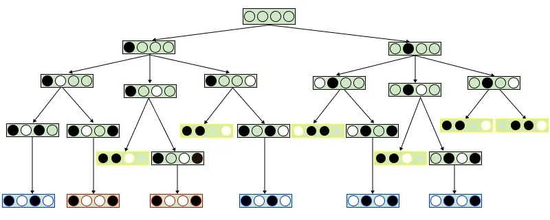
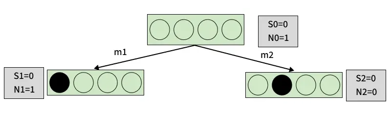
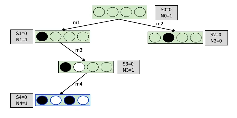
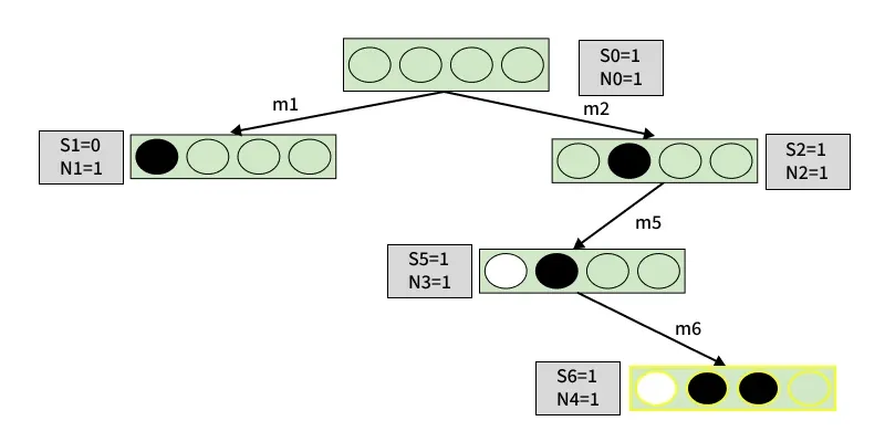
Monte Carlo Tree Search Example

Game: Pair

• Players: 2
• Board: 4 boxes
• Winning Condition: A player wins by marking any two adjacent boxes.

The full game tree contains three types of terminal (leaf) states:

• Yellow leaves: Winning positions (+1) -> Total: 6 nodes
• Blue leaves: Draw positions (0) -> Total: 4 nodes
• Red leaves: Losing positions (–1) -> Total: 2 nodes

These values will be used during simulation and backpropagation.

Iteration 1

1. Selection & Expansion

• Start at root S0; two moves m1 and m2 lead to S1 and S2.
• Compute UCB for S1 and S2. Both are unvisited leaf nodes -> UCB = -> pick randomly -> select S1.

2. Simulation (from S₁)

• Roll out randomly from S1 to a terminal state.
• One playout (moves m3, m4) ends in a draw (0).
• Record: e.g., S4 = 0, N4 = 1.

3. Backpropagation

Backpropagate the 0 result along the path to S0 (update values/visits on each node).

Iteration 2

1. Selection

Now we compare S1 and S2:

• S1 has been visited once -> finite UCB
• S2 not visited -> UCB =

So we select S2.

2. Simulation (from S2)

• Roll out randomly from S2.
• One playout (moves m5, m6) ends in a win (+1).
• Record: e.g., S6 = +1, N6 = 1.

3. Backpropagation

Update values along the path:

• Value(S2) = 1
• Visits(S2) = 1

The root now has results from both S1 and S2.

Iteration 3

1. Selection

• After two interactions, both S1 and S2 have N = 1.
• UCB favors S2 (it has a win), so select S2 again.

Python Implementation

1. Importing Libraries

We will start by importing required libraries:

• math: to perform mathematical operations like logarithms and square roots for UCB1 calculations.
• random: to randomly pick moves during simulations (rollouts).
• deepcopy: to safely copy board state

2. check_winner_state(state)

Checks if any player (1 or 2) has won. Returns:

• 1: Player 1 wins
• 2: Player 2 wins
• None: No winner

3. available_actions(state)

Returns all empty cells (i, j) where a move can be placed.

4. get_current_player(state)

Determines whose turn it is by counting Xs and Os.

• If equal: Player 1
• Else: Player 2

5. MCTS Node Class

Each node represents a game state in the search tree.

• state: 3×3 board
• parent: previous node
• action: move applied at the parent to get here
• player: who made that move
• children: child nodes
• visits: number of times this node was visited
• wins: total reward from simulations
• untried_actions: moves not explored yet

6. Helper Function

• is_terminal(): Checks if the game is finished.
• is_fully_expanded(): Returns True if all moves are explored.
• expand(): Takes one untried move → creates a child node → adds it to the tree.
• best_child(): Selects the best child using UCB1 formula (exploitation + exploration).

7. rollout()

Plays random moves until the game finishes. Returns:

• 1 or 2: winner
• None: draw

8. backpropagate()

Updates the wins and visits from simulation results.

9. MCTS Search Function

Runs the complete MCTS process:

• Selection
• Expansion
• Simulation
• Backpropagation

10. Playing the Game (MCTS vs Random)

11. Run the Game

Output:

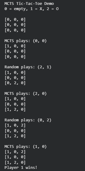
With enough iterations, MCTS plays strong and avoids losing lines. Increasing simulation count improves decision quality. A real-world example is AlphaGo, which combined MCTS with neural networks and achieved world-class performance by running millions of simulations per move.

Practical Applications Beyond Games

1. Planning and Scheduling: The algorithm can optimize resource allocation and task scheduling in complex systems where traditional optimization methods struggle.
2. Neural Architecture Search: MCTS guides the exploration of neural network architectures, helping to discover optimal designs for specific tasks.
3. Portfolio Management: Financial applications use MCTS for portfolio optimization under uncertainty, where the algorithm balances risk and return through simulated market scenarios.

Advantages

• No domain knowledge needed: MCTS only needs valid moves and end conditions.
• Balances exploration and exploitation: Uses UCB to pick promising and less-explored moves.
• Anytime algorithm: Can stop at any moment and still return the best estimated move.
• Works well with large search spaces: Focuses on useful parts of the tree instead of exploring everything.
• Asymmetric tree growth: Spends more time on good branches, improving decision quality efficiently.

Limitations

• Simulation-heavy: needs many rollouts for consistent results
• High variance: random rollouts can lead to noisy estimates
• Tactical blindness: may miss short forced sequences
• Parameter tuning: exploration constant (c) impacts results