Non-Linear SVM - ML

Support Vector Machines (SVM) are algorithms for classification and regression tasks. However, the standard (linear) SVM can only classify data that is linearly separable, meaning a straight line can separate the classes (in 2D) or a hyperplane (in higher dimensions). Non-linear SVM extends SVM to handle complex, non-linearly separable data using kernels.

For example, imagine classifying fruits like apples and oranges based on features like colour and texture. The apple data points might form a circular cluster surrounded by oranges. A simple SVM can’t separate them, but a non-linear SVM handles this by using kernel functions to create curved boundaries, allowing it to classify such complex, non-linear patterns accurately.

Kernel

Instead of explicitly transforming data, the kernel computes dot products in a higher-dimensional space, helping the model find patterns and separate complex data more easily. For example, suppose we have data points shaped like two concentric circles:

• One circle represents one class.
• The other circle represents another class.

If we try to separate these classes with a straight line it can't be done because the data is not linearly separable in its current form.

When we use a kernel function it transforms the original 2D data like the concentric circles into a higher-dimensional space where the data becomes linearly separable. In that higher-dimensional space the SVM finds a simple straight-line decision boundary to separate the classes.

When we bring this straight-line decision boundary back to the original 2D space it no longer looks like a straight line. Instead, it appears as a circular boundary that perfectly separates the two classes. This happens because the kernel trick allows the SVM to "see" the data in a new way enabling it to draw a boundary that fits the original shape of the data.

Popular kernel functions in SVM

• Radial Basis Function (RBF): Captures patterns in data by measuring the distance between points and is ideal for circular or spherical relationships. It is widely used as it creates flexible decision boundary.
• Linear Kernel: Works for data that is linearly separable problem without complex transformations.
• Polynomial Kernel: Models more complex relationships using polynomial equations.
• Sigmoid Kernel: Uses a sigmoid function similar to neural networks but is less commonly used in practice, as it may not satisfy all mathematical conditions (positive semi-definiteness) for every parameter setting.

Below are some examples of Non-Linear SVM Classification.

Example 1: Non linear SVM in Circular Decision Boundary

Below is the Python implementation for Non linear SVM in circular decision boundary.

1. Importing Libraries

We begin by importing the necessary libraries for data generation, model training, evaluation and visualization.

2. Creating and Splitting the Dataset

We generate a synthetic dataset of concentric circles and split it into training and testing sets.

3. Creating and Training the Non-Linear SVM Model

We create an SVM classifier using the RBF kernel to handle non-linear patterns and train it on the data.

4. Making Predictions and Evaluating the Model

We predict the labels for the test set and compute the accuracy of the model.

5. Visualizing the Decision Boundary

We define a function to visualize the decision boundary of the trained non-linear SVM on the dataset.

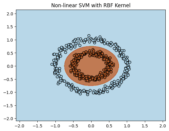
Output:

Non linear SVM provided a decision boundary where the SVM successfully separates the two circular classes (inner and outer circles) using a curved boundary with help of RBF kernel.

Example 2: Non linear SVM for Interleaving Half-Moon Data

Now we will see how different kernel works. We will be using polynomial kernel function for dataset with interleaving half-moon pattern.

1. Importing Libraries

We import essential libraries for dataset creation, SVM modeling, evaluation and visualization.

2. Creating and Splitting the Dataset

We generate a synthetic "two moons" dataset which is non-linearly separable and split it into training and test sets.

3. Creating and Training the SVM with Polynomial Kernel

We build an SVM classifier with a polynomial kernel and train it on the training data.

4. Making Predictions and Evaluating the Model

We use the trained model to predict test labels and evaluate its accuracy.

5. Visualizing the Decision Boundary

We define a function to plot the decision boundary learned by the SVM with a polynomial kernel.

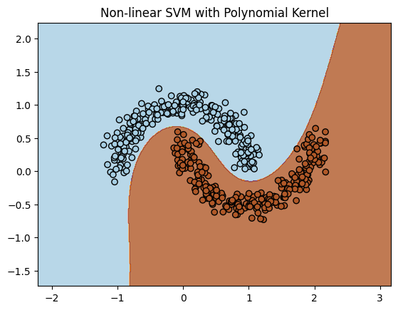
Output:

Polynomial kernel creates a smooth, non-linear decision boundary that effectively separates the two curved regions.

Linear SVM vs Non-Linear SVM

Applications

1. Image Classification: They are widely used for image recognition tasks such as handwritten digit recognition like MNIST dataset where the data classes are not linearly separable.
2. Bioinformatics: Used in gene expression analysis and protein classification where the relationships between variables are complex and non-linear.
3. Natural Language Processing (NLP): Used for text classification tasks like spam filtering or sentiment analysis where non-linear relationships exist between words and sentiments.
4. Medical Diagnosis: Effective for classifying diseases based on patient data such as tumor classification where data have non-linear patterns.
5. Fraud Detection: They can identify fraudulent activities by detecting unusual patterns in transactional data.
6. Voice and Speech Recognition: Useful for separating different voice signals or identifying speech patterns where non-linear decision boundaries are needed.