Role of KL-divergence in Variational Autoencoders

Variational Autoencoders

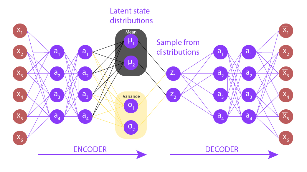
Variational autoencoder was proposed in 2013 by Knigma and Welling at Google and Qualcomm. A variational autoencoder (VAE) provides a probabilistic manner for describing an observation in latent space. Thus, rather than building an encoder that outputs a single value to describe each latent state attribute, we’ll formulate our encoder to describe a probability distribution for each latent attribute.

Architecture:

Autoencoders basically contains two parts: 

• The first one is an encoder which is similar to the convolution neural network except for the last layer. The aim of the encoder is to learn efficient data encoding from the dataset and pass it into a bottleneck architecture.
• The other part of the autoencoder is a decoder that uses latent space in the bottleneck layer to regenerate the images similar to the dataset. These results backpropagate from the neural network in the form of the loss function.

Variational autoencoder is different from autoencoder in a way such that it provides a statistical manner for describing the samples of the dataset in latent space. Therefore, in the variational autoencoder, the encoder outputs a probability distribution in the bottleneck layer instead of a single output value.

👁 Image

Explanation:

The Variational Autoencoder latent space is continuous. It provides random sampling and interpolation. Instead of outputting a vector of size n, the encoder outputs two vectors:

• Vector ????  of means (vector size n)
• Vector ???? of standard deviations (vector size n)

Output is an approximate posterior distribution q(z|x). Sample from this distribution to get z. let's look at more details into Sampling:

• Let's take some values of mean and standard deviation,
• The intermediate distribution that is generated from that:
• Now, let's generate the sampled vector from this:
• While the mean and standard deviation are the same for one input the result may be different due to sampling.
• Eventually, our goal is to make the encoder learn to generate differently???? For different classes, clustering them and generating encoding such they don't vary much. To this we use KL-divergence.

KL-divergence:

KL divergence stands for Kullback Leibler Divergence, it is a measure of divergence between two distributions. Our goal is to Minimize KL divergence and optimize ???? and ???? of one distribution to resemble the required distribution.Of  

For multiple distribution the KL-divergence can be calculated as the following formula:

where X_j \sim N(\mu_j, \sigma_j^{2})  is the standard normal distribution.

VAE Loss:

Suppose we have a distribution z and we want to generate the observation x from it.  In other words, we want to calculate 

 

We can do it by following way:

 

But, the calculation of p(x) can be quite difficult

 

This usually makes it an intractable distribution. Hence, we need to approximate p(z|x) to q(z|x) to make it a tractable distribution. To better approximate p(z|x) to q(z|x), we will minimize the KL-divergence loss which calculates how similar two distributions are:

 

By simplifying, the above minimization problem is equivalent to the following maximization problem :

 

The first term represents the reconstruction likelihood and the other term ensures that our learned distribution q is similar to the true prior distribution p.

Thus our total loss consists of two terms, one is reconstruction error and the other is KL-divergence loss:

Implementation:

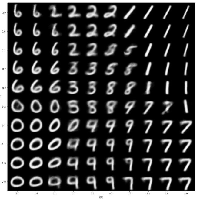
In this implementation, we will be using the MNIST dataset, this dataset is already available in keras.datasets API, so we don't need to add or upload manually.

• First, we need to import the necessary packages to our python environment. we will be using Keras package with TensorFlow as a backend.

• For variational autoencoders, we need to define the architecture of two parts encoder and decoder but first, we will define the bottleneck layer of architecture, the sampling layer.

• Now, we define the architecture of the encoder part of our autoencoder, this part takes images as input and encodes their representation in the Sampling layer.

Model: "encoder"
__________________________________________________________________________________________________
Layer (type) Output Shape Param # Connected to 
==================================================================================================
input_3 (InputLayer) [(None, 28, 28, 1)] 0 
__________________________________________________________________________________________________
conv2d_2 (Conv2D) (None, 14, 14, 32) 320 input_3[0][0] 
__________________________________________________________________________________________________
conv2d_3 (Conv2D) (None, 7, 7, 64) 18496 conv2d_2[0][0] 
__________________________________________________________________________________________________
flatten_1 (Flatten) (None, 3136) 0 conv2d_3[0][0] 
__________________________________________________________________________________________________
dense_2 (Dense) (None, 16) 50192 flatten_1[0][0] 
__________________________________________________________________________________________________
z_mean (Dense) (None, 2) 34 dense_2[0][0] 
__________________________________________________________________________________________________
z_log_var (Dense) (None, 2) 34 dense_2[0][0] 
__________________________________________________________________________________________________
sampling_1 (Sampling) (None, 2) 0 z_mean[0][0] 
 z_log_var[0][0] 
==================================================================================================
Total params: 69, 076
Trainable params: 69, 076
Non-trainable params: 0
__________________________________________________________________________________________________

• Now, we define the architecture of decoder part of our autoencoder, this part takes the output of the sampling layer as input and output an image of size (28, 28, 1) . 

Model: "decoder"
_________________________________________________________________
Layer (type) Output Shape Param # 
=================================================================
input_4 (InputLayer) [(None, 2)] 0 
_________________________________________________________________
dense_3 (Dense) (None, 3136) 9408 
_________________________________________________________________
reshape_1 (Reshape) (None, 7, 7, 64) 0 
_________________________________________________________________
conv2d_transpose_3 (Conv2DTr (None, 14, 14, 64) 36928 
_________________________________________________________________
conv2d_transpose_4 (Conv2DTr (None, 28, 28, 32) 18464 
_________________________________________________________________
conv2d_transpose_5 (Conv2DTr (None, 28, 28, 1) 289 
=================================================================
Total params: 65, 089
Trainable params: 65, 089
Non-trainable params: 0
_________________________________________________________________

• In this step, we combine the model and define the training procedure with loss functions. 

• Now it's the right time to train our variational autoencoder model, we will train it for 100 epochs.  But first we need to import the MNIST dataset.

• In this step, we display training results, we will be displaying these results according to their values in latent space vectors.

👁 Image

• To get a more clear view of our representational latent vectors values, we will be plotting the scatter plot of training data on the basis of their values of corresponding latent dimensions generated from the encoder  

 
 

👁 Image

 

• To compare the difference, I also train the above autoencoder for \beta =0 i.e we remove the Kl-divergence loss, and it generated the following distribution:

👁 Image

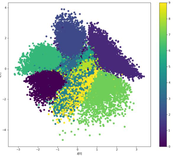
Here, we can see that the distribution is not separable and quite skewed for different values, that's why we use KL-divergence loss in the above variational autoencoder.

References:

• Variational Autoencoder Paper
• Keras Variational Autoencoder