Different Loss functions in SGD

In machine learning, optimizers and loss functions are two components that help improve the performance of the model. A loss function measures the performance of a model by measuring the difference between the output expected from the model and the actual output obtained from the model. Mean square loss and log loss are some examples of loss functions. The optimizer helps to improve the model by adjusting its parameters so that the loss function value is minimized. SGD, ADAM, and RMSProp are some examples of optimizers. The focus of this article will be the various loss functions supported by the SGD module of Sklearn. Sklearn provides two classes of SGD: SGDClassifier for classification tasks and SGDRegressor for regression tasks.

SGD Optimizer

Stochastic Gradient Descent (SGD) is a variant of the gradient descent algorithm. Gradient descent is an iterative optimization technique used to minimize a given loss function and find the global minimum or maximum. This loss function can take various forms, as long as it is differentiable. Here's a breakdown of the process:

1. Data Standardization: Begin by standardizing the input data.
2. Parameter Initialization: Initialize the model's parameters and hyperparameters, like the learning rate.
3. Derivative Computation: Calculate the derivatives of the loss with respect to the model's parameters.
4. Parameter Update: Update the model's parameters iteratively until you reach the global minimum of the loss function.

Gradient descent has a drawback when dealing with large datasets. It requires using the entire training dataset to update the model's parameters. When dealing with millions of records, this process becomes slow and computationally expensive.

Stochastic Gradient Descent (SGD) addresses this issue by using only a single randomly selected data point (or a small batch of data points) to update the parameters in each iteration. However, SGD still suffers from slow convergence because it necessitates performing forward and backward propagation for every individual data point. Additionally, this approach leads to a noisy path toward the global minimum.

SGD Classifier Loss Function

The SGD classifier supports the following loss functions:

Hinge Loss: Support Vector Machine

Hinge loss serves as a loss function in training of classifiers. It is employed specifically in 'maximum margin' classification with SVMs being a prominent example.

Mathematically, Hinge loss can be represented as :

Here,

• t - the actual output (class ) required from the classifier(true class)
• y - the raw output of the classifier or classifier score (not the predicted class)

Lets understand it with the help of below graph:

👁 Hinge loss-gfg

We can identify three cases in the loss function

Case 1: Correct Classification and |y| ≥ 1

In this case the product t.y will always be positive and its value greater than 1 and therefore the value of 1-t.y will be negative. So, the loss function value max(0,1-t.y) will always be zero. This is indicated by the green region in above graph. Here there is no penalty to the model.

Case 2: Correct Classification and |y| < 1

In this case the product t.y will always be positive, but its value will be less than 1 and therefore the value of 1-t.y will be positive with value ranging between 0 to 1. Hence the loss function value will be the value of 1-t.y. This is indicated by the yellow region in above graph. Here though the model has correctly classified the data we are penalizing the model because it has not classified it with much confidence (|y| < 1) as the classification score is less than 1.

Case 3: Incorrect Classification

In this case the product t.y will always be negative therefore the value of 1-t.y will be always positives. So the loss function value max(0,1-t.y) will always be the value given by 1-t.y. Here the loss value will increase linearly with increase in value of y. This is indicated by the red region in above graph.

Modified Huber Loss: Smoothed Hinge Loss

Huber loss is a loss function used in regression. Its variant for classification is called as modified Huber loss.

Mathematically the Huber Loss can be expressed as

if, and otherwise.

Here,

• t - the actual output (class ) required from the classifier(true class)
• y - the raw output of the classifier or classifier score (not the predicted class)

The modified Huber loss can be graphically represented as:

👁 Modified Hinge Loss-gfg

For values of yt > -1 (the light red, yellow and green area in the graph) it is basically hinge loss squared.

For values of yt <-1 the loss function value is -4yt indicated by the dark red area in graph.

Log Loss: Logistic Regression

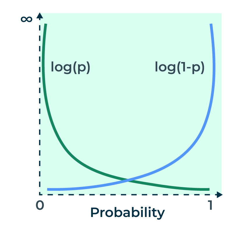
Log loss or binary entropy loss is the loss function used for logistic regression.

Mathematically, it can be expressed as:

Here, we have two classes - Class 1 and Class 0

• p = probability of the datapoint belonging to class 1
• is the class label (1 for Class 1 and 0 for Class 0)

Case Class 1: Second term in the equation becomes 0 and we will be left with first term only.

Case Class 0: First term in the equation becomes 0 an wee will be left with the second term only.

Let us understand the log loss with the help of graph:

👁 Log Loss for individual data point -gfg

Class 1 - The green line represents Class 1. When the predicted probability is close to 1, the loss approaches zero and when the predicted probability is close to 0, loss approaches infinity.

Class 0 - The blue line represents Class 0. When the predicted probability is close to 0, the loss approaches zero and when the predicted probability is close to 1, loss approaches infinity.

Note the above the graph is the log loss for individual data point and not for the whole equation. Actual loss is obtained by summing the loss values of individual data point and it depends on the probability value .

SGD Regressor Loss Functions

SGD regressor supports the following loss functions.

Squared Error: Ordinary Least Squares

The ordinary least squares is the square of the difference between the actual value and predicted value.

The lost function can be mathematically be expressed as:

Here,

• y- it is the actual value
• f(x) - it is value predicted by the model

It tends to penalize model more and more for larger differences thereby giving more weight to outliers

Graphically, it can be represented for one point as below:

👁 Squared Error-gfg

Huber Loss: Robust Regression

The mean squared error (MSE) or squared error gives too much importance to outliers and Mean Average error (MAE) (here instead of squaring we take absolute value of errors) gives equal weightage to all points. Huber loss combines MSE and MAE to give best of both wold- it is quadratic(MSE) when the error is small else MAE. For a loss value less than delta we use MSE and for loss value greater then delta we use MAE. The delta value is a hyperparameter.

The equation of Huber loss is given by:

Here,

• y = observed value
• = predicted value
  

The use of delta in the second part of the equation is to make the equation differentiable and continuous.

👁 Huber Loss-gfg

Epsilon Insensitive: Linear Support Vector Regression

The epsilon insensitive loss can be mathematically be expressed as:

Here,

• - the actual output (class ) required from the classifier(true class)
• - the raw output of the classifier or classifier score (not the predicted class)

The value of epsilon determines the distance within which errors are considered to be zero . The loss function ignores error which are less than or equal to epsilon value by treating them zero.

Thus the loss function effectively forces the optimizer to find such a hyperplane that a tube of width epsilon around this hyperplane will contain all the datapoints.

Implementing Different SGD Loss Functions in Python

Classification

• Import Necessary Libraries

Load the IRIS Dataset

Split in Train and Test Set

Model training using Hinge Loss

• We have imported SGD Classifier from scikit-learn and specified the loss function as 'hinge'.
• Model uses the training data and corresponding labels to classify data based on hinge loss function.

Model Evaluation when, loss = 'hinge'

Output:

Hinge Loss
Precision score : 0.98125
Recall score : 0.98
Confusion Matrix
array([[19, 0, 0],
 [ 0, 15, 1],
 [ 0, 0, 15]])

Model training and evaluation using Modified Huber Loss

• We have imported SGD Classifier from scikit-learn and specified the loss function as 'modified_huber'.
• Model uses the training data and corresponding labels to classify data based on modified huber loss function.

Output:

Modified Huber
Precision score : 0.9520000000000001
Recall score : 0.76
Confusion Matrix
array([[19, 3, 0],
 [ 0, 3, 0],
 [ 0, 9, 16]])

Model training and evaluation using Log Loss

• We have imported SGD Classifier from scikit-learn and specified the loss function as 'log_loss'.
• Model uses the training data and corresponding labels to classify data based on log loss function.

Output:

Log Loss
Precision score : 0.9413333333333332
Recall score : 0.78
Confusion Matrix
array([[19, 2, 0],
 [ 0, 4, 0],
 [ 0, 9, 16]])

Regression

Import necessary libraries

Load California Housing Dataset

Split the dataset in test and train

Scaling the training and test set

Model training and evaluation using Squared Error Loss function

• We have specified the loss function as squared error. The model uses the training data and the corresponding target values. The model will learn to predict the target values using squared error loss.
• We will use the trained model to make predictions on the test data.
• Coefficient of determination measures how well the model fits the data. It represents the proportion of the variance in the target variable that is explained by the model.

Output:

Squared Error
Coefficient of determination: 0.9128269523492567

Model training and evaluation using Huber Loss function

• We have specified the loss function as Huber loss function. The model uses the training data and the corresponding target values.

Output:

Huber Error
Coefficient of determination: 0.9148961830574946

Model training and evaluation using Epsilon Insensitive Loss function

• We have specified the loss function as Epsilon Insensitive function. The model uses the training data and the corresponding target values.

Output:

Epsilon Insensitive Loss Function
Coefficient of determination: 0.4266448634462471