Train a model using CatBoost

CatBoost is the current one of the state-of-the-art ML models that can be used both for the regression as well as the classification task. By the name, we can say that the cat boost models were built taking into consideration the fact that they will be used to deal with the datasets that have categorical columns in them. In this article, we will learn how can we train a CatBoost model for the classification purpose on the placement data that has been taken from the Kaggle.

Catboost

Catboost (Categorical Boosting), is a high-performance, open-source, gradient-boosting framework developed by Yandex. It is intended to address a broad spectrum of machine learning problems, such as regression, ranking, and classification, with a focus on effectively managing categorical information. Catboost is unique in the structured data processing space because of its speed, accuracy, and user-friendliness.

How Catboost Works?

A high-performance gradient-boosting method designed for machine learning applications, particularly those requiring structured input, is called Catboost. Its primary mechanism is based on the ensemble learning technique known as gradient boosting. Typically, Catboost starts by speculating on the target variable's mean. The next step is to progressively build the ensemble of decision trees, with each tree aiming to remove the residuals or errors from the preceding one. The way that Catboost manages category features makes it unique. Catboost processes categorical data directly using an approach known as "ordered boosting," which improves model performance and speeds up training.

To prevent overfitting, regularization strategies are also included. When generating predictions, Catboost combines thе forecasts from every tree, producing incredibly dependablе and precise models. Furthermore, it provides feature relevance rankings that facilitate thе understanding of model choices and thе selection of features. For many different machine-learning tasks, including regression and classification, Catboost is a helpful tool.

Implementation Using CatBoost

!pip install catboost

Importing Libraries and Dataset

Python libraries make it very easy for us to handle the data and perform typical and complex tasks with a single line of code.

• Pandas – This library helps to load the data frame in a 2D array format and has multiple functions to perform analysis tasks in one go.
• Numpy – Numpy arrays are very fast and can perform large computations in a very short time.
• Matplotlib/Seaborn – This library is used to draw visualizations.
• Sklearn – This module contains multiple libraries having pre-implemented functions to perform tasks from data preprocessing to model development and evaluation.
• We'll use this dataset to perform a classification task using the catboost algorithm.

First step first we will load the data into the pandas dataframe.

Output:

 StudentID CGPA Internships Projects Workshops/Certifications \
0 1 7.5 1 1 1 
1 2 8.9 0 3 2 
2 3 7.3 1 2 2 
3 4 7.5 1 1 2 
4 5 8.3 1 2 2 
 AptitudeTestScore SoftSkillsRating ExtracurricularActivities \
0 65 4.4 No 
1 90 4.0 Yes 
2 82 4.8 Yes 
3 85 4.4 Yes 
4 86 4.5 Yes 
 PlacementTraining SSC_Marks HSC_Marks PlacementStatus 
0 No 61 79 NotPlaced 
1 Yes 78 82 Placed 
2 No 79 80 NotPlaced 
3 Yes 81 80 Placed 
4 Yes 74 88 Placed 

If we take a moment to understand the data first then we will get to know that this dataset contains information about the students academic and training and placement status.

• CGPA - It is the overall grades achieved by the student.
• Internships - It tells the number of internships a student has done.
• Projects - Numbe rof projects a student has done.
• Workshops/Certifications - As there are multiple MOOC courses available online student opt for them to upskill themselves.
• ApptitudeTestScore - Aptitude test are generally a part of the recruitment process to understand the Quant and logical thinking of the student.
• SoftSkillrating - Communication is a key role that plays in the placement or in any aspect of the life.
• ExtraCurricularActivities - This helps provide and insight about the personality of an individual regarding how much he is active other than the academic.
• PlacementTraining - It is provided to students in college to ace teh placement process.
• SSC and HSC - Senior Secondary and Higher Secondary Marks.
• PlacementStatus - This is our target column with two classes placed and not placed.

So, this is all about the dataset now let's check the shape of the dataset to know how many data entries have been provided to us.

Output:

(10000, 12)

By using the df.info() function we can see the content of each columns and the data types present in it along with the number of null values present in each column.

Output:

<class 'pandas.core.frame.DataFrame'>
RangeIndex: 10000 entries, 0 to 9999
Data columns (total 12 columns):
 # Column Non-Null Count Dtype 
--- ------ -------------- ----- 
 0 StudentID 10000 non-null int64 
 1 CGPA 10000 non-null float64
 2 Internships 10000 non-null int64 
 3 Projects 10000 non-null int64 
 4 Workshops/Certifications 10000 non-null int64 
 5 AptitudeTestScore 10000 non-null int64 
 6 SoftSkillsRating 10000 non-null float64
 7 ExtracurricularActivities 10000 non-null object 
 8 PlacementTraining 10000 non-null object 
 9 SSC_Marks 10000 non-null int64 
 10 HSC_Marks 10000 non-null int64 
 11 PlacementStatus 10000 non-null object 
dtypes: float64(2), int64(7), object(3)
memory usage: 937.6+ KB

The DataFrame df is described statistically via the df.describe() function. In order to provide a preliminary understanding of the data's central tendencies and distribution, it includes important statistics such as count, mean, standard deviation, minimum, and maximum values for each numerical column.

Output:

 count mean std min 25% \
StudentID 10000.0 5000.50000 2886.895680 1.0 2500.75 
CGPA 10000.0 7.69801 0.640131 6.5 7.40 
Internships 10000.0 1.04920 0.665901 0.0 1.00 
Projects 10000.0 2.02660 0.867968 0.0 1.00 
Workshops/Certifications 10000.0 1.01320 0.904272 0.0 0.00 
AptitudeTestScore 10000.0 79.44990 8.159997 60.0 73.00 
SoftSkillsRating 10000.0 4.32396 0.411622 3.0 4.00 
ExtracurricularActivities 10000.0 0.58540 0.492677 0.0 0.00 
PlacementTraining 10000.0 0.73180 0.443044 0.0 0.00 
SSC_Marks 10000.0 69.15940 10.430459 55.0 59.00 
HSC_Marks 10000.0 74.50150 8.919527 57.0 67.00 
PlacementStatus 10000.0 0.41970 0.493534 0.0 0.00 
 50% 75% max 
StudentID 5000.5 7500.25 10000.0 
CGPA 7.7 8.20 9.1 
Internships 1.0 1.00 2.0 
Projects 2.0 3.00 3.0 
Workshops/Certifications 1.0 2.00 3.0 
AptitudeTestScore 80.0 87.00 90.0 
SoftSkillsRating 4.4 4.70 4.8 
ExtracurricularActivities 1.0 1.00 1.0 
PlacementTraining 1.0 1.00 1.0 
SSC_Marks 70.0 78.00 90.0 
HSC_Marks 73.0 83.00 88.0 
PlacementStatus 0.0 1.00 1.0 

Exploratory Data Analysis

EDA is an approach to analyzing the data using visual techniques. It is used to discover trends, and patterns, or to check assumptions with the help of statistical summaries and graphical representations. While performing the EDA of this dataset we will try to look at what is the relation between the independent features that is how one affects the other.

Now let's start with a short analysis of the null values in the data frame column wise.

Output:

StudentID 0
CGPA 0
Internships 0
Projects 0
Workshops/Certifications 0
AptitudeTestScore 0
SoftSkillsRating 0
ExtracurricularActivities 0
PlacementTraining 0
SSC_Marks 0
HSC_Marks 0
PlacementStatus 0
dtype: int64

So, we are good to go for the data exploration as there are no null values in the dataset.

DIstributions of Target Class

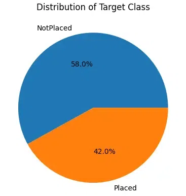
Output:

👁 Target Class Distributions-Geeksforgeeks

From the above pie chart of the distribution of the classes in the dataset is nearly balanced it is not perfect but yeah it is acceptable. We can observe that there are categorical columns as well as numerical columns in the dataset let's separate them in two list before we move on to the analysis of these features.

Output:

Categorical : ['Internships', 'Projects', 'Workshops/Certifications', 'ExtracurricularActivities', 'PlacementTraining', 'PlacementStatus']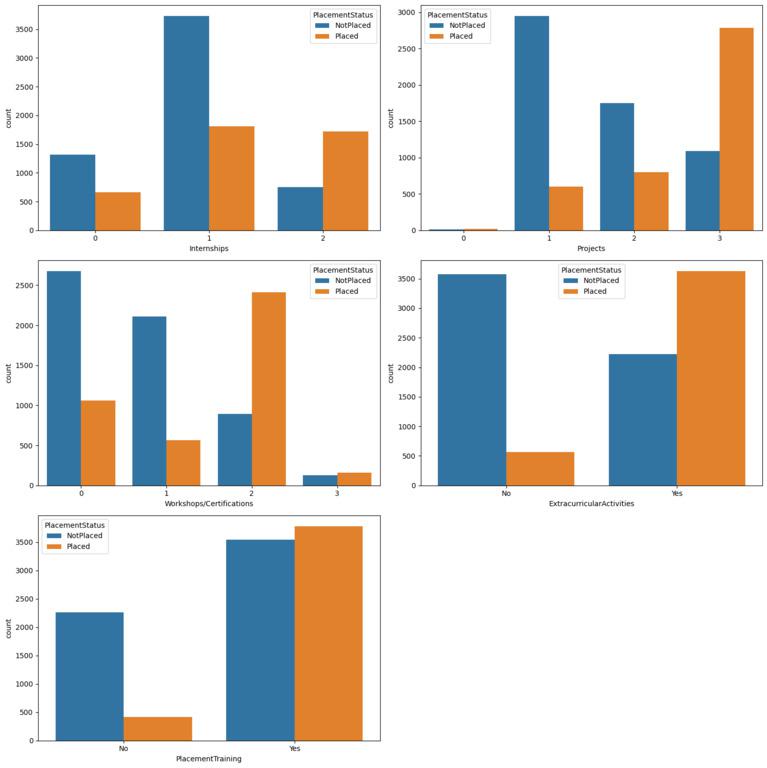
Numerical : ['StudentID', 'CGPA', 'AptitudeTestScore', 'SoftSkillsRating', 'SSC_Marks', 'HSC_Marks']

Countplot for categorical columns

Now, let's create countplot for the categorical columns with the hue of the placement status.

Output:

👁 img5

From the above charts we can observe multiple patterns that empower the fact that the work done on your skill development will definitely help you get placed. There are certainly cases where the students have completed training programs and projects but still they are not placed but the ratio of them is quite low as compare to that who has done nothing.

Label Encoding of Categorical Columns

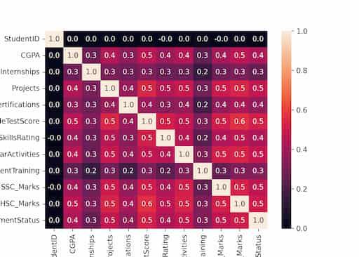
Now as we have encoded the categorical features in the dataset let's create a heatmap that can be used to identify the highly correlated features with the target columns of within the feature space itself.

Confusion Matrix

Output:

👁 Confusion Matrix-Geeksforgeeks

From here we can observe that there are no highly correlated feature in the dataset so, no data leakage and correlated features.

Train & Validations Data Split

To evaluate the performance of the model while the training process goes on let's split the dataset in 85:15 ratio. This will help us evaluate the performance of the model by using the unseen dataset of the validation split.

Output:

((8500, 10), (1500, 10))

Feature scaling

This code fits the StandardScaler to the training data to calculate the mean and standard deviation and then transforms both the training and validation data using these calculated values to ensure consistent scaling between the two datasets.

Now we are ready to train the model using the training data that we have prepared. Here we are performing binary classification as the target column that is Y_train and Y_val have 0 and 1 only that means binary classification task also it is not necessary to specify separately while training the model weather it is for the binary classification task or the multi-class classification.

Build and Train the Model

To avoid the overfitting we can tune some of the hyperparameters of the model.

• Iterations: We can define the custom number of iterations to train our model on the data for. This can be helpful to avoid the overfitting when the size of the dataset is small.
• loss_function: Using this hyperparameter we can define the loss function that we would like to use to train our model on.
• early_stopping_rounds: This hyperparameter is useful when we have splitter our data into training and the validation dataset. This stops further training of the model when the model starts overfitting the training data.
• custom_metric: This can be used to print the performance of the model on the custom metric as the training process goes on.

Output:

Learning rate set to 0.053762
0: learn: 0.6621731 test: 0.6623146 best: 0.6623146 (0) total: 1.58ms remaining: 1.58s
100: learn: 0.3971504 test: 0.4332513 best: 0.4331288 (92) total: 158ms remaining: 1.41s
Stopped by overfitting detector (50 iterations wait)bestTest = 0.4331287949
bestIteration = 92Shrink model to first 93 iterations.

Now let's check the performance of the model using the ROC-AUC metric on the training and the validation data.

Output:

Training ROC-AUC: 0.8140948743198752
Validation ROC-AUC: 0.7850069999416671

Conclusion

In conclusion, the model has been trained using Catboost algorithm. The algorithm has shown to be a highly effective way for binary classification tasks.