What is Lag in Time Series Forecasting

Time series forecasting is a crucial aspect of predictive modeling, often used in fields like finance, economics, and meteorology. It involves using historical data points to predict future trends. One important concept within time series analysis is lag, which plays a significant role in understanding and modeling the relationship between past and future values in a time series.

In this article, we will explore the concept of lag in time series forecasting, its importance, and how it is applied in forecasting models.

Overview of Time Series Forecasting

Before diving into the concept of lag, let’s briefly understand time series forecasting. A time series is a sequence of data points collected or recorded at regular time intervals. The primary goal of time series forecasting is to predict future values based on previously observed values. This is widely used in predicting stock prices, sales, weather, and more.

Forecasting models utilize various techniques such as moving averages, exponential smoothing, and autoregressive integrated moving average (ARIMA) models. A critical part of these models is how they use historical data to make predictions, which brings us to the concept of lag.

Understanding Lag in Time Series

In time series analysis, lag refers to the delay between an observed data point and its preceding values. Specifically, lag is the time difference between two observations in a sequence, or the number of steps back in time a past observation is from the current time.

Example of Lag:

Let’s consider a simple time series representing the monthly sales of a company over five months:

In this example:

• Lag 1 would compare the sales in month 2 (220 units) with the sales in month 1 (200 units).
• Lag 2 would compare the sales in month 3 (230 units) with the sales in month 1 (200 units).

Thus, a lag of 1 refers to the immediate previous observation, a lag of 2 refers to two steps back, and so on.

Importance of Lag in Forecasting

Lag is important because it helps to identify patterns and relationships between past and present data points. Time series models, such as ARIMA, heavily rely on lag to capture autocorrelations (the correlation between observations at different time lags) in the data.

Key reasons why lag is essential:

• Autocorrelation Detection: Lag enables analysts to understand how current data points are related to previous ones. If there is a significant autocorrelation at a particular lag, it suggests that past values can be used to predict future values.
• Feature Creation: In machine learning models for time series forecasting, lagged variables are often used as features. These features represent the values of the time series at previous time steps, allowing the model to learn patterns over time.
• Trend Identification: By observing how values change across different lags, trends and seasonality can be identified. For instance, a consistent increase in lagged values may indicate an upward trend.

Types of Lag in Time Series

There are several types of lag used in time series analysis, depending on the relationship being analyzed:

1. Simple Lag: This is the most basic form of lag, where each observation is compared with its previous values. It is often used to detect basic patterns like trends or seasonality.
2. Lagged Difference: Lagged difference involves subtracting the current value from the value at a previous lag. This helps to stabilize the mean of a time series and make it stationary. For instance, if the difference between sales in month 3 and month 1 is significant, lagged difference can reveal this.
3. Lag Operators: Lag operators are mathematical notations used to represent lag in time series models. For instance, in ARIMA models, the lag operator "L" is used to denote lagged values, where refers to lag 1, refers to lag 2, and so on.

Lag in ARIMA Models

The Autoregressive Integrated Moving Average (ARIMA) model is one of the most commonly used time series models that leverage lag. In ARIMA, the model forecasts a time series based on the linear relationship between an observation and a number of lagged observations.

• Autoregressive (AR) Component: This component models the relationship between an observation and lagged observations. The number of lagged terms (p) is selected to optimize the forecast.
• Moving Average (MA) Component: The MA component models the relationship between an observation and the residual errors of lagged observations.

In the ARIMA model, determining the optimal number of lags (the parameter p) is critical for accurate predictions.

How to Select Lag in Time Series Forecasting

Selecting the optimal lag is crucial to ensure accurate forecasting. There are a few common techniques to identify the best lag for time series models:

1. Autocorrelation Function (ACF)

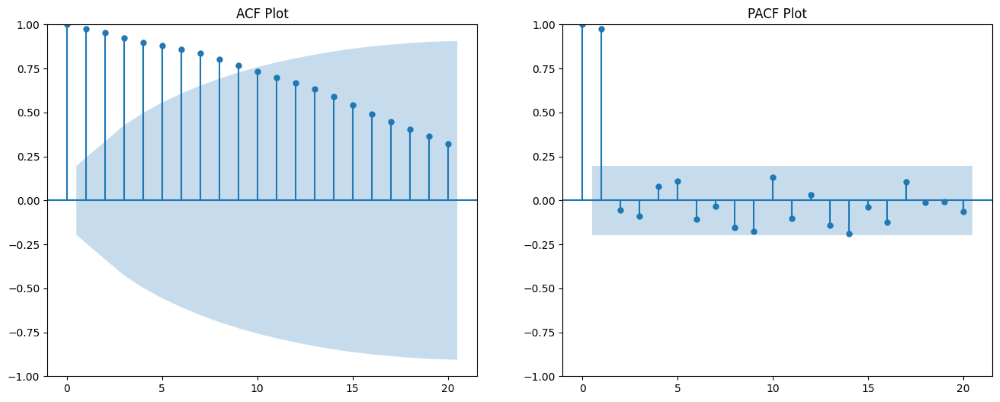
TheAutocorrelation Function (ACF) helps to measure the correlation between an observation and its lagged values. The ACF plot shows the strength of correlation across different lags. If a series has strong correlations at specific lags, those lags can be considered for use in the model.

• Use case: ACF is typically used to determine the number of moving average (MA) terms in ARIMA models.

2. Partial Autocorrelation Function (PACF)

The Partial Autocorrelation Function (PACF) measures the correlation between an observation and its lagged observations while controlling for the correlations of all shorter lags. The PACF plot helps to find the direct relationship between a variable and its past values, filtering out the intermediate lags.

• Use case: PACF is primarily used to determine the number of autoregressive (AR) terms in ARIMA models.

3. Information Criteria (AIC/BIC)

The Akaike Information Criterion (AIC) and Bayesian Information Criterion (BIC) are statistical metrics that evaluate model performance. These metrics penalize complex models and help in selecting the optimal lag by fitting models with different lags and comparing their AIC/BIC scores. The model with the lowest score is preferred.

• Use case: AIC/BIC is useful when selecting optimal lag values in ARIMA or other autoregressive models.

4. Grid Search

In some cases, performing a grid search for different lag values and comparing model accuracy can be beneficial. This involves trying multiple lag combinations and selecting the one with the best performance based on accuracy metrics like Mean Squared Error (MSE) or Root Mean Squared Error (RMSE).

Implementation: Selecting Optimal Lag in Time Series Forecasting Using ACF, PACF, and AIC

To select the optimal lag in time series forecasting, we can use autocorrelation plots and statistical methods like Partial Autocorrelation Function (PACF) or Autocorrelation Function (ACF) plots. In Python, the statsmodels library provides tools for performing these tasks.

Here’s how you can implement and choose the optimal lag in Python using ACF, PACF, and information criteria (like AIC):

Step 1: Import Required Libraries

Step 2: Load Time Series Data

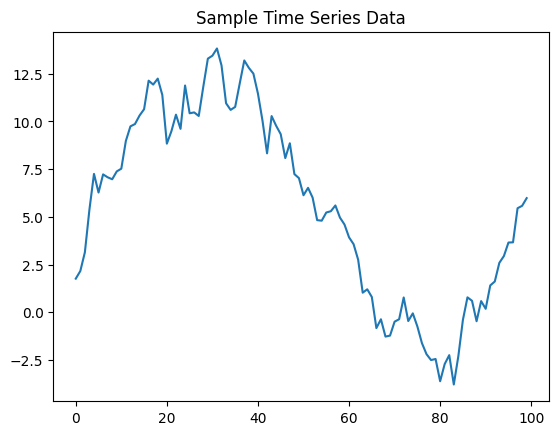
For this example, we will use a simple time series. You can replace it with your dataset.

Output:

Step 3: Visualize ACF and PACF to Determine Lag

You can use the Autocorrelation Function (ACF) and Partial Autocorrelation Function (PACF) plots to visually select the optimal lag for an ARIMA model.

Output:

• ACF Plot helps to see how each point in the series correlates with previous points (useful for determining MA terms).
• PACF Plot helps to see the direct relationship between an observation and a lagged observation (useful for determining AR terms).

Step 4: Using Information Criteria (AIC/BIC) for Lag Selection

Alternatively, you can use Akaike Information Criterion (AIC) or Bayesian Information Criterion (BIC) to choose the optimal lag by fitting ARIMA models with different lags and comparing the AIC/BIC scores.

Output:

Lag: 1, AIC: 290.97158925836254
Lag: 2, AIC: 292.3695498699307
Lag: 3, AIC: 292.63569462782016
Lag: 4, AIC: 294.6330969513839
Lag: 5, AIC: 296.07875295289756
Lag: 6, AIC: 297.6370086026085
Lag: 7, AIC: 298.9122341233797
Lag: 8, AIC: 296.61311484062776
Lag: 9, AIC: 294.7954409798874
Lag: 10, AIC: 294.25539005911094

Optimal Lag based on AIC: 1

Challenges in Working with Lag

While lag is a powerful tool in time series forecasting, it comes with certain challenges:

• Choosing the Right Lag: Determining the optimal number of lags to include in a model can be difficult. Too few lags may lead to underfitting, while too many can cause overfitting.
• Stationarity: Time series data often need to be stationary (i.e., having a constant mean and variance over time) for effective lag-based modeling. Non-stationary data may require transformations, such as differencing, to remove trends or seasonality.

Conclusion

Lag in time series forecasting is a fundamental concept that helps to establish relationships between past and future values. By incorporating lagged observations into forecasting models, analysts can capture patterns, detect trends, and make more accurate predictions.

Whether using simple lag, lag operators, or advanced models like ARIMA, understanding how lag works is key to effective time series analysis. However, selecting the right lag and managing challenges like stationarity are crucial for ensuring the accuracy and robustness of forecasts.