Ridge Regression is a version of linear regression that adds an L2 penalty to control large coefficient values. While Linear Regression only minimizes prediction error, it can become unstable when features are highly correlated. Ridge solves this by shrinking coefficients making the model more stable and reducing overfitting. It helps in:

• L2 Regularization: Adds an L2 penalty to model weights
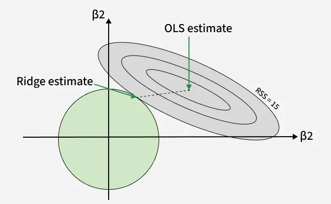
• Bias-Variance Tradeoff: Controls how large coefficients can grow
• Multicollinearity: Improves stability when features overlap
• Generalization: Helps the model generalize better on new data

Bias-Variance Trade-off in Ridge Regression

One of the central ideas behind ridge regression is the bias-variance trade-off:

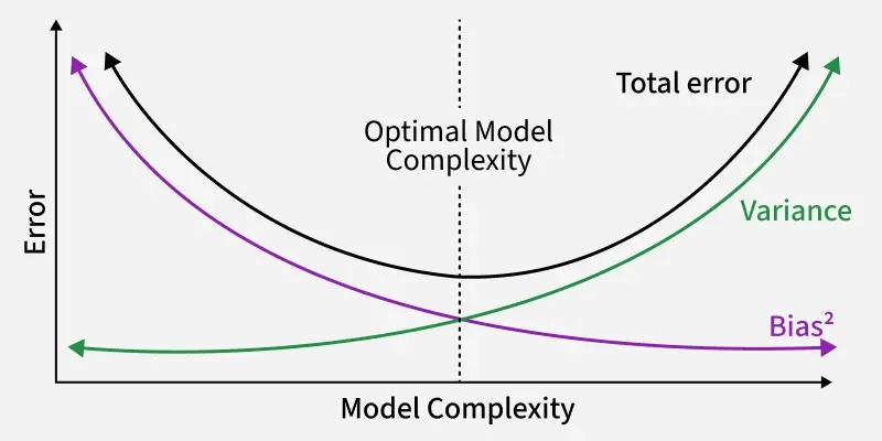
• Variance: In standard linear regression, especially when features are correlated or many, coefficient estimates can vary a lot depending on the specific training data, meaning predictions on new data can be very unstable.
• Bias: Ridge regression deliberately introduces some bias by shrinking coefficient magnitudes. This means the fit to the training data might be slightly worse.
• Trade-off & Why It Helps: Ridge shrinks large coefficients hence reducing variance. Even with a small increase in bias, the overall MSE drops, giving better performance than plain linear regression on new data.

Thus, ridge regression accepts a small increase in bias to gain a larger reduction in variance and this tradeoff is often useful when generalization is important.

Selection of the Ridge Parameter

Choosing the right ridge parameter k is essential because it directly affects the model’s bias-variance balance and overall predictive accuracy. Several systematic approaches exist for determining the optimal value of k, each offering unique strengths and considerations. The major methods are:

1. Cross-Validation

Cross-validation selects the ridge parameter by repeatedly training and testing the model on different subsets of data and identifying the value of k that minimizes validation error.

• K-Fold Cross-Validation: The dataset is divided into K folds. The model trains on K–1 folds and validates on the remaining fold. This process repeats for all folds and the average error determines the best k.
• Leave-One-Out Cross-Validation (LOOCV): A special form of cross-validation where each observation acts once as the validation point. Though computationally expensive, it provides an almost unbiased estimate of prediction error.

2. Generalized Cross-Validation (GCV)

It is an efficient alternative to LOOCV that avoids explicitly splitting the data. It estimates the optimal k by minimizing a function that approximates the LOOCV error.

• Requires fewer computations.
• Often produces results similar to traditional cross-validation.

3. Information Criteria

Model selection metrics like AIC and BIC can also guide the choice of k.

• They balance model fit with complexity.
• Higher penalties discourage overly complex or over-regularized models.

4. Empirical Bayes Methods

These methods treat k as a Bayesian hyperparameter and use observed data to estimate its value.

• Empirical Bayes Estimation: A prior distribution is assigned to k and the data are used to update it into a posterior distribution. The posterior mean or mode is then selected as the optimal k.

5. Stability Selection

Stability selection enhances robustness by repeatedly fitting the model on subsampled datasets.

• The ridge parameter that appears most consistently across subsamples is chosen.
• Helps avoid unstable or overly sensitive parameter choices.

Implementation

Let's implement it and here we will import numpy and scikit learn.

• StandardScaler: Ensures all features are on the same scale so the ridge penalty affects them fairly.
• alpha (λ) in Ridge Regression: Controls the strength of regularization hence larger values shrink coefficients more aggressively.
• Train-test split: Divides data into training and testing sets to evaluate generalization performance.
• Ridge(alpha=1.0): Initializes a Ridge Regression model with a chosen regularization parameter.
• ridge.fit(): Fits the model to training data and estimates the coefficients under L2 penalty.
• ridge.predict(): Uses the trained model to generate predictions on unseen test data.
• mean_squared_error(): Measures the average squared difference between predicted and actual values; lower is better.
• GridSearchCV: Systematically tests multiple alpha values to find the one that minimizes error using cross-validation.
• best_estimator_: The model with the optimal alpha found through GridSearchCV.
• coef_: The final learned coefficients after applying L2 shrinkage.

Output:

Applications

• Multicollinearity Handling: Stabilizes estimates when predictors are highly correlated.
• High-Dimensional Data: Performs well when the number of features is large or exceeds observations.
• Noise-Resistant Modeling: Reduces variance and improves prediction on noisy datasets.
• Domain Usage: Common in finance, econometrics, genomics and marketing analytics.
• ML Workflow Integration: Serves as a strong baseline regularized regression model.

Advantages

• Overfitting Control: Shrinks coefficients to prevent the model from memorizing noise.
• Correlation Support: Handles correlated predictors more effectively than linear regression.
• Better Generalization: Produces stable predictions on new, unseen data.
• Feature Retention: Keeps all features in the model instead of dropping any unlike Lasso.

Limitations

• No Feature Selection: Coefficients are shrunk but never reduced to exact zero.
• Hyperparameter Sensitivity: Requires careful λ (alpha) tuning for best performance.
• Irrelevant Feature Impact: May still be affected when many inputs add no useful information.
• Reduced Interpretability: Heavy shrinkage can obscure the true effect of predictors.
• Poor Fit for Sparse Models: Not ideal when only a few predictors truly matter.