seaborn.countplot() in Python

seaborn.countplot() is a function in the Seaborn library in Python used to display the counts of observations in categorical data. It shows the distribution of a single categorical variable or the relationship between two categorical variables by creating a bar plot. Example:

Output :

Explanation: This code creates a count plot using Seaborn to display the frequency of male and female individuals in the sex column of the "tips" dataset. It uses sns.countplot() to plot the data and plt.show() to display the plot.

Syntax

seaborn.countplot(x=None, y=None, hue=None, data=None, order=None, hue_order=None, orient=None, color=None, palette=None, saturation=0.75, dodge=True, ax=None, **kwargs)

Parameters:

• x, y: This parameter take names of variables in data or vector data, optional, Inputs for plotting long-form data.
• hue : (optional) This parameter take column name for colour encoding.
• data : (optional) This parameter take DataFrame, array, or list of arrays, Dataset for plotting. If x and y are absent, this is interpreted as wide-form. Otherwise it is expected to be long-form.
• order, hue_order : (optional) This parameter take lists of strings. Order to plot the categorical levels in, otherwise the levels are inferred from the data objects.
• orient : (optional)This parameter take “v” | “h”, Orientation of the plot (vertical or horizontal). This is usually inferred from the dtype of the input variables but can be used to specify when the “categorical” variable is a numeric or when plotting wide-form data.
• color : (optional) This parameter take matplotlib color, Color for all of the elements, or seed for a gradient palette.
• palette : (optional) This parameter take palette name, list, or dict, Colors to use for the different levels of the hue variable. Should be something that can be interpreted by color_palette(), or a dictionary mapping hue levels to matplotlib colors.
• saturation : (optional) This parameter take float value, Proportion of the original saturation to draw colors at. Large patches often look better with slightly desaturated colors, but set this to 1 if you want the plot colors to perfectly match the input color spec.
• dodge : (optional) This parameter take bool value, When hue nesting is used, whether elements should be shifted along the categorical axis.
• ax : (optional) This parameter take matplotlib Axes, Axes object to draw the plot onto, otherwise uses the current Axes.
• kwargs : This parameter take key, value mappings, Other keyword arguments are passed through to matplotlib.axes.Axes.bar().

Return Value: Returns the Axes object with the plot drawn onto it.

Examples of seaborn.countplot()

Example 1: Show value counts for two categorical variables and using hue parameter

This code demonstrates how to create a count plot using Seaborn in Python to visualize the distribution of categorical data. We are using the "tips" dataset from Seaborn, and the plot visualizes the frequency of male and female customers (sex) while distinguishing between smokers and non-smokers using the hue parameter.

Output:

Explanation: In this code, sns.countplot() is used to create a count plot where the x-axis represents the sex column, and the hue parameter splits the data by smoker status. The plt.show()function renders the plot, displaying the distribution of male and female customers as well as how many of them smoke or don't smoke.

Example 2: Plot the bars horizontally

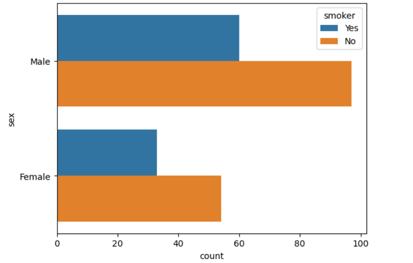
This code demonstrates how to create a count plot using Seaborn in Python with the "tips" dataset. Unlike the standard vertical count plot, this code uses the y parameter to plot the categorical variable (sex) on the y-axis.

Output:

Explanation: In this code, sns.countplot() is used with the y parameter to create a horizontal count plot. The y-axis represents the sex column, while the hue parameter divides the data based on whether the customers are smokers or not. The plt.show() function displays the plot, allowing us to compare the number of male and female customers who smoke versus those who do not.

Example 3: Use different color palette attributes 

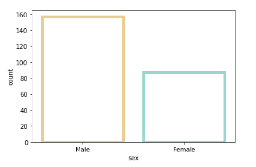
This code shows how to use a custom color palette in a Seaborn count plot. The "tips" dataset is loaded using Seaborn, and the count plot visualizes the distribution of male and female customers (sex). By using the palette parameter with the "Set2" palette, we change the default colors of the plot to create a visually appealing and distinguishable chart.

Output:

Explanation: In this code, sns.countplot() is used to create a vertical bar plot of the sex column from the "tips" dataset. The palette parameter is set to "Set2", which is a predefined Seaborn color palette, to style the plot with a specific set of colors. The plot displays the count of male and female customers, and plt.show() is used to render the plot.

Possible values of palette are:

Accent, Accent_r, Blues, Blues_r, BrBG, BrBG_r, BuGn, BuGn_r, BuPu, BuPu_r, CMRmap, CMRmap_r, Dark2, Dark2_r,
GnBu, GnBu_r, Greens, Greens_r, Greys, Greys_r, OrRd, OrRd_r, Oranges, Oranges_r, PRGn, PRGn_r, Paired, Paired_r,
Pastel1, Pastel1_r, Pastel2, Pastel2_r, PiYG, PiYG_r, PuBu, PuBuGn, PuBuGn_r, PuBu_r, PuOr, PuOr_r, PuRd, PuRd_r,
Purples, Purples_r, RdBu, RdBu_r, RdGy, RdGy_r, RdPu, RdPu_r, RdYlBu, RdYlBu_r, RdYlGn, RdYlGn_r, Reds, Reds_r, Set1,
Set1_r, Set2, Set2_r, Set3, Set3_r, Spectral, Spectral_r, Wistia, Wistia_r, YlGn, YlGnBu, YlGnBu_r, YlGn_r, YlOrBr,
YlOrBr_r, YlOrRd, YlOrRd_r, afmhot, afmhot_r, autumn, autumn_r, binary, binary_r, bone, bone_r, brg, brg_r, bwr, bwr_r,
cividis, cividis_r, cool, cool_r, coolwarm, coolwarm_r, copper, copper_r, cubehelix, cubehelix_r, flag, flag_r, gist_earth,
gist_earth_r, gist_gray, gist_gray_r, gist_heat, gist_heat_r, gist_ncar, gist_ncar_r, gist_rainbow, gist_rainbow_r, gist_stern, 

Example 4: using a color parameter in the plot.

This code demonstrates how to create a count plot using Seaborn to visualize the distribution of passengers by class in the Titanic dataset. The plot also differentiates between male and female passengers using the hue parameter.

Output:

Explanation: In this code, sns.countplot() is used to create a count plot that shows the number of passengers in each class (class) from the Titanic dataset. The hue parameter is set to 'sex', which splits the bars based on male and female passengers. The color parameter is set to "salmon" to change the bar colors. The plt.show() function displays the resulting plot.

Example 5: Using a saturation parameter in the plot.

This code demonstrates how to create a count plot using Seaborn, visualizing the distribution of male and female passengers from the Titanic dataset. The color parameter is set to "salmon", and the saturation is adjusted to 0.1 for a lighter color tone.

Output:

Explanation: In this code, the sns.countplot() function is used to create a count plot showing the number of male and female passengers (sex) from the Titanic dataset. The color parameter is set to "salmon" to color the bars. The saturation parameter is set to 0.1, which reduces the intensity of the color, making it lighter. The plt.show() function is called to display the plot.

Example 6: Use matplotlib.axes.Axes.bar() parameters to control the style.

This code demonstrates how to create a count plot using Seaborn for the 'sex' column in the Titanic dataset. Custom edge colors and transparency are applied to the bars, enhancing the plot's visual appearance.

Output:

Explanation: In this code, the sns.countplot() function is used to create a count plot for the 'sex' column in the Titanic dataset. The color parameter is set to "salmon", while facecolor=(0, 0, 0, 0) makes the bars transparent. The linewidth is set to 5, making the edges thicker. The edgecolor is customized using a color palette ("BrBG", 2) for a distinct visual appeal. Finally, plt.show() displays the plot.

Colormap Possible values are:  

Accent, Accent_r, Blues, Blues_r, BrBG, BrBG_r, BuGn, BuGn_r, BuPu, BuPu_r,  
CMRmap, CMRmap_r, Dark2, Dark2_r, GnBu, GnBu_r, Greens, Greens_r, Greys, Greys_r,  
OrRd, OrRd_r, Oranges, Oranges_r, PRGn, PRGn_r, Paired, Paired_r, Pastel1, Pastel1_r,  
Pastel2, Pastel2_r, PiYG, PiYG_r, PuBu, PuBuGn, PuBuGn_r, PuBu_r, PuOr, PuOr_r, PuRd,
PuRd_r, Purples, Purples_r, RdBu, RdBu_r, RdGy, RdGy_r, RdPu, RdPu_r, RdYlBu, RdYlBu_r,
RdYlGn, RdYlGn_r, Reds, Reds_r, Set1, Set1_r, Set2, Set2_r, Set3, Set3_r, Spectral,