How to split the Dataset With scikit-learn's train_test_split() Function

In this article, we will discuss how to split a dataset using scikit-learns' train_test_split().

sklearn.model_selection.train_test_split() function:

The train_test_split() method is used to split our data into train and test sets. First, we need to divide our data into features (X) and labels (y). The dataframe gets divided into X_train, X_test, y_train, and y_test. X_train and y_train sets are used for training and fitting the model. The X_test and y_test sets are used for testing the model if it's predicting the right outputs/labels. we can explicitly test the size of the train and test sets. It is suggested to keep our train sets larger than the test sets.

• Train set: The training dataset is a set of data that was utilized to fit the model. The dataset on which the model is trained. This data is seen and learned by the model.
• Test set: The test dataset is a subset of the training dataset that is utilized to give an accurate evaluation of a final model fit.
• validation set:  A validation dataset is a sample of data from your model's training set that is used to estimate model performance while tuning the model's hyperparameters.
• underfitting: A data model that is under-fitted has a high error rate on both the training set and unobserved data because it is unable to effectively represent the relationship between the input and output variables.
• overfitting:  when a statistical model matches its training data exactly but the algorithm's goal is lost because it is unable to accurately execute against unseen data is called overfitting

Syntax: sklearn.model_selection.train_test_split(*arrays, test_size=None, train_size=None, random_state=None, shuffle=True, stratify=None

Parameters:

• *arrays: sequence of indexables. Lists, numpy arrays, scipy-sparse matrices, and pandas dataframes are all valid inputs.
• test_size: int or float, by default None. If float, it should be between 0.0 and 1.0 and represent the percentage of the dataset to test split. If int is used, it refers to the total number of test samples. If the value is None, the complement of the train size is used. It will be set to 0.25 if train size is also None.
• train_size: int or float, by default None.
• random_state : int,by default None. Controls how the data is shuffled before the split is implemented. For repeatable output across several function calls, pass an int.
• shuffle: boolean object , by default True. Whether or not the data should be shuffled before splitting. Stratify must be None if shuffle=False.
• stratify: array-like object , by default it is None. If None is selected, the data is stratified using these as class labels.

Returns:

splitting: The train-test split of inputs is represented as a list.

Steps to split the dataset:

Step 1: Import the necessary packages or modules:

In this step, we are importing the necessary packages or modules into the working python environment.

Step 2: Import the dataframe/ dataset:

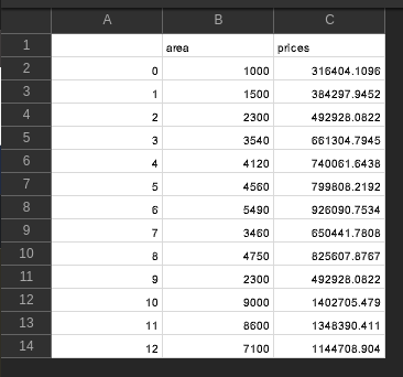
Here, we load the CSV using pd.read_csv() method from pandas and get the shape of the data set using the shape() function.

CSV Used:

👁 Image

Output:

(13, 3)

Step 3: Get X and Y feature variables:

Here, we are assigning the X and the Y variable in which the X feature variable has independent variables and the y feature variable has a dependent variable.

Step 4: Use the train test split class to split data into train and test sets:

Here, the train_test_split() class from sklearn.model_selection is used to split our data into train and test sets where feature variables are given as input in the method. test_size determines the portion of the data which will go into test sets and a random state is used for data reproducibility.

Example:

In this example, 'predictions.csv' file is imported. df.shape attribute is used to retrieve the shape of the data frame. The shape of the dataframe is (13,3). The features columns are taken in the X variable and the outcome column is taken in the y variable. X and y variables are passed in the train_test_split() method to split the data frame into train and test sets. The random state parameter is used for data reproducibility. test_size is given as 0.25 which means 25% of the data goes into the test sets. 4 out of 13 rows in the dataframe go into the test sets. 75% of data goes into the train sets, which is 9 rows out of 13 rows. The train sets are used to fit and train the machine learning model. The test sets are used for evaluation.

CSV Used:

👁 Image

Output:

(13, 3)
Head of the dataframe : 
 Unnamed: 0 area prices
0 0 1000 316404.109589
1 1 1500 384297.945205
2 2 2300 492928.082192
3 3 3540 661304.794521
4 4 4120 740061.643836
Index(['Unnamed: 0', 'area', 'prices'], dtype='object')
X_train : 
3 3540
7 3460
4 4120
0 1000
8 4750
Name: area, dtype: int64
(9,)

X_test : 
12 7100
2 2300
11 8600
10 9000
Name: area, dtype: int64
(4,)

y_train : 
3 661304.794521
7 650441.780822
4 740061.643836
0 316404.109589
8 825607.876712
Name: prices, dtype: float64
(9,)

y_test : 
12 1.144709e+06
2 4.929281e+05
11 1.348390e+06
10 1.402705e+06
Name: prices, dtype: float64
(4,)

Example:

In this example the following steps are executed :

• The necessary packages are imported.
• Advertising.csv data set is loaded and cleaned, and null values are dropped.
• feature and target arrays are created(X andy).
• The arrays created are split into train and test sets. 30% of the dataset goes into the test set, which means 70% data is a train set.
• A standard scaler object is created.
• X_train is fit into the scaler.
• X_train and X_test are transformed using the transform() method.
• A simple linear regression model is created
• Train sets fit in the model.
• the predict() method is used to carry out predictions on the X_test set.
• mean_squared_error() metric is used to evaluate the model.

To view and download the CSV file used in this example, click here. 

Output:

array([19.82000933, 14.23636718, 12.80417236,  7.75461569,  8.31672266,

       15.4001915 , 11.6590983 , 15.22650923, 15.53524916, 19.46415132,

       17.21364106, 16.69603229, 16.46449309, 10.15345178, 13.44695953,

       24.71946196, 18.67190453, 15.85505154, 14.45450049,  9.91684409,

       10.41647177,  4.61335238, 17.41531451, 17.31014955, 21.72288151,

        5.87934089, 11.29101265, 17.88733657, 21.04225992, 12.32251227,

       14.4099317 , 15.05829814, 10.2105313 ,  7.28532072, 12.66133397,

       23.25847491, 18.87101505,  4.55545854, 19.79603707,  9.21203026,

       10.24668718,  8.96989469, 13.33515217, 20.69532628, 12.17013119,

       21.69572633, 16.7346457 , 22.16358256,  5.34163764, 20.43470231,

        7.58252563, 23.38775769, 10.2270323 , 12.33473902, 24.10480458,

        9.88919804, 21.7781076 ])

2.7506859249500466

Example:

In this example, we're gonna use the K-nearest neighbors classifier model. 

In this example the following steps are executed :

• The necessary packages are imported.
• iris data is loaded from sklearn.datasets.
• feature and target arrays are created(X andy).
• The arrays created are split into train and test sets. 30% of the dataset goes into the test set, which means 70% data is a train set.
• A basic Knn model is created using the KNeighborsClassifier class.
• Train sets fit in the knn model.
• the predict() method is used to carry out predictions on the X_test set.

Output:

[1 0 2 1 1 0 1 2 1 1 2 0 0 0 0 1 2 1 1 2 0 2 0 2 2 2 2 2 0 0]