 |
VOOZH | about |
|
VOOZH | about |
In science and engineering, many problems involve quantities that change over time like speed of a moving object or temperature of a cooling cup. These changes are often described using differential equations.
SciPy provides a function called odeint (from the scipy.integrate module) that helps solve these equations numerically. By giving it a function that describes how your system changes and some starting values, odeint calculates how the system behaves over time.
scipy.integrate.odeint (func, y0, t, args=())
Parameter:
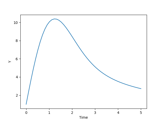
Let's solve an ordinary differential equation (ODE) using the odeint() function.
Output
Explanation:
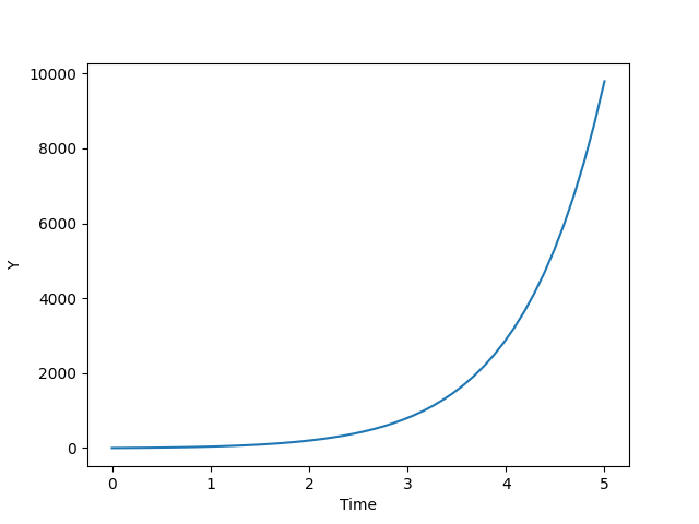
Output
Explanation:
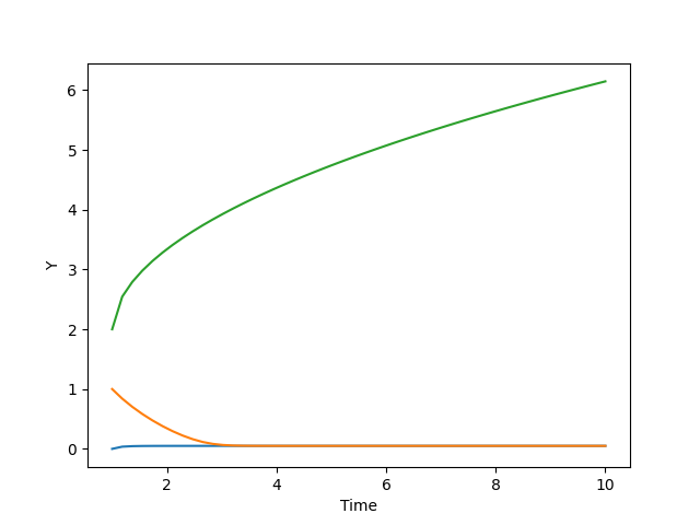
Output
Explanation: