Time Series Decomposition Techniques

Time series data consists of observations recorded over time, such as daily stock prices, monthly sales, or yearly temperatures. Time series decomposition helps in:

• Understanding long-term trends.
• Identifying repeating seasonal patterns.
• Detecting random fluctuations or anomalies.

Here, we will learn about the types of decomposition, common methods, and how to implement them in Python with examples.

Components of a Time Series

A time series can be split into three main components:

• Trend: Represents the long-term movement in the data. For Example, gradual increase in sales over years.
• Seasonality: Represents repeating patterns over fixed periods, like daily, weekly, or yearly cycles. For Example, ice cream sales rising every summer.
• Residual (Noise): Random fluctuations that remain after removing trend and seasonality. For Example, unexpected sales spike due to a one-time event.

Types of Time Series Decomposition

Additive Decomposition: In additive decomposition, the time series is expressed as the sum of its components:

Y(t)=Trend(t)+Seasonal(t)+Residual(t)

It's suitable when the magnitude of seasonality doesn't vary with the magnitude of the time series.

Multiplicative Decomposition: In multiplicative decomposition, the time series is expressed as the product of its components:

Y(t)=Trend(t)×Seasonal(t)×Residual(t)

It's suitable when the magnitude of seasonality scales with the magnitude of the time series.

Methods of Decomposition

1. Moving Averages: Moving averages involve calculating the average of a certain number of past data points. It helps smooth out fluctuations and highlight trends.
2. Seasonal Decomposition of Time Series: The Seasonal and Trend decomposition using Loess (STL) is a popular method for decomposition, which uses a combination of local regression (Loess) to extract the trend and seasonality components.
3. Exponential Smoothing State Space Model: This method involves using the ETS framework to estimate the trend and seasonal components in a time series.

Implementation

Let's go through an example of applying multiple time series decomposition techniques to a sample dataset. We'll use Python and some common libraries.

Step 1: Import the required libraries.

We have imported the following libraries:

• NumPy: Numeric computations
• Pandas: Data manipulation
• Matplotlib: Visualization
• Statsmodels: Time series decomposition and analysis

Step 2: Create a Synthetic Time Series Dataset

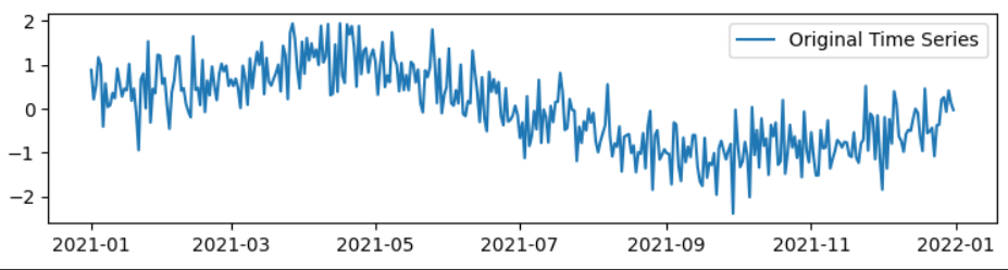
To demonstrate decomposition, we create a sample time series resembling real-world data. It combines a sine wave (to simulate seasonal patterns) with random noise, producing daily observations over one year.

Output

2021-01-01 0.882026
2021-01-02 0.217292
2021-01-03 0.523791
2021-01-04 1.172066
2021-01-05 1.002581
...
2021-12-27 0.263264
2021-12-28 -0.066917
2021-12-29 0.414305
2021-12-30 0.135561
2021-12-31 -0.025054
Freq: D, Length: 365, dtype: float64

Step 3: Visualize the Time Series

Plot the original time series to inspect its patterns over time:

Output

Step 4: Apply Additive Decomposition

The following code uses the seasonal_decomposition function from the Statsmodels library to decompose the original time series (ts) into its constituent components using an additive model.

Syntax of seasonal_decompose:

seasonal_decompose(x, model='additive', filt=None, period=None, two_sided=True, extrapolate_trend=0)

We can also set model='multiplicative' but, our data contains zero and negative values. Hence, we are only going to proceed with the additive model.

The code performs an additive decomposition of the original time series and stores the result in the result_add variable, allowing you to further analyze and visualize the decomposed components.

Step 5: Plot Trend Component

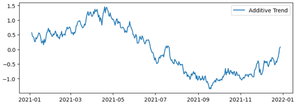
Visualize the trend extracted from the additive decomposition to observe the long-term movement in the data.

Output

👁 trend-

Step 6: Plot the Seasonal Component

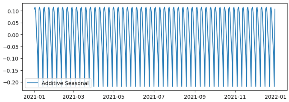
Visualize the seasonal pattern extracted from the additive decomposition to see repeating short-term fluctuations:

Output

👁 seasonal--min

Step 7: Calculate the Simple Moving Average (SMA)

The provided code calculates a simple moving average (SMA) for the original time series (ts) with a 7-day moving window

Output

2021-01-01 NaN
2021-01-02 NaN
2021-01-03 NaN
2021-01-04 NaN
2021-01-05 NaN
...
2021-12-27 -0.326866
2021-12-28 -0.262944
2021-12-29 -0.142060
2021-12-30 0.030998
2021-12-31 0.081171
Freq: D, Length: 365, dtype: float64

Step 8: Calculate Exponential Moving Average (EMA)

The provided code calculates an exponential moving average (EMA) for the original time series (ts) with a 30-day window.

Output

2021-01-01 0.882026
2021-01-02 0.839140
2021-01-03 0.818795
2021-01-04 0.841587
2021-01-05 0.851973
...
2021-12-27 -0.428505
2021-12-28 -0.405176
2021-12-29 -0.352307
2021-12-30 -0.320831
2021-12-31 -0.301749
Freq: D, Length: 365, dtype: float64

Step 9: Plot Moving Averages

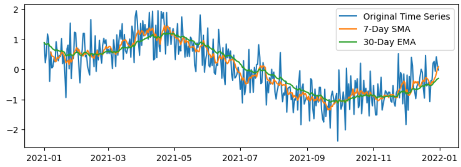
The following code creates a plot that overlays the original time series (ts) with the 7-day Simple Moving Average (SMA) and the 30-day Exponential Moving Average (EMA), highlighting both short-term and long-term trends.

Output

👁 ema-sma-