Some Advanced OpenCV Operations For Your Computer vision Project!

This article was published as a part of the Data Science Blogathon

Introduction.

Computer Vision is said to be one of the most interesting application fields of Machine Learning. Computer Vision. As implied by the name, Computer Vision enables computers to detect, identify, and recognize, objects and patterns in the 3D surroundings.

If you have not viewed my previous articles on Computer Vision and would like to do so, kindly navigate to the following hyperlinks:

• Article
  1: An Introduction to Computer Vision With OpenCV.
• Article
  2: Performing Computer Vision Task With OpenCV And Python.

This article will introduce you to more features of the OpenCV Library.

Source: Analytics Vidhya.

Recap

As we seek to explore more about the world of OpenCV, let us take a moment to recap, or brush up, on what we have learned up to this point.

• We have obtained a short, general insight into what is Machine Learning?
• We have been introduced to the OpenCV Library.
• We are aware that our implementation of OpenCV is in Python Programming
  Language.
• We loaded an image into system memory and observed an image in two different colour formats, viz., standard (default) and GRAYSCALE.
• We understand the base nature in which OpenCV represents images, i.e., The NumPy Array comprising integers, representing pixel intensity. Up to this point, we have only looked at a GRAYSCALE image.
• We viewed a few important properties of the image array such as the contents, shape, and type of data.

OpenCV Python Programming.

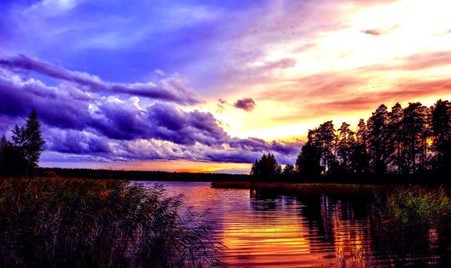
We understand exactly how to load an image into the system’s main memory. We will now look at more complex operations that can be performed on image data. To facilitate this OpenCV learning experience we will be using an image that may be downloaded from this link. Alternatively, you may save the image found below.

Source: Pinterest.

Loading The Image.

The first and foremost step will be to load the image into our system memory as follows:

import cv2
 # load it in GRAYSCALE color mode...
 image = cv2.imread("""C:/Users/Shivek/Pictures/cd0c13629f217c1ab72c61d0664b3f99.jpg""", 0)
 cv2.imshow('Analytics Vidhya Computer Vision- Nature.png Gray', image)
 cv2.waitKey()
 cv2.destroyAllWindows()

C:/Users/Shivek/Pictures/cd0c13629f217c1ab72c61d0664b3f99.jpg 

The above code successfully loads the required image into our system memory. It is good to know that we
have loaded the image in GRAYSCALE colour format.

(Explanation to the above code will be omitted as it is the same as the previous article(s).

Output to the above code block will be seen as below:

Obtaining and Understanding Image Properties.

Let us gain insight into our image by viewing the associated properties. We will now talk about the shape of the image.

print(image.shape)

Output is as below:

Notice that the shape method returns two values to us in the form of a tuple. These two values represent the height (y-axis) and width (x-axis) of the image, respectively. Essentially what I am saying is:

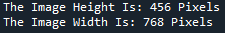
print("The Image Height Is: %d Pixels"%(image.shape[0]))
 print("The Image Width Is: %d Pixels"%(image.shape[1]))

Output to the above code is
as below:

There are some situations in which the shape method returns a tuple of three integer values. The first value represents the height (y-axis), the second value the width (x-axis), and the third value, the number of color channels.

Colour channels affect the colour ranges (i.e., Types/Shades of colours | Reds, Blues, Pinks, etc.) of your pixels. Taking our example, we have a GRAYSCALE image- A GRAYSCALE image has
just one color channel because each element in the pixel array contains just
one value that ranges from 0 to 255.

Looking at Image Color Channels.

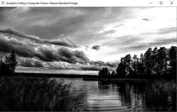
For example, and experience purposes, let us re-load our nature image, and view the shape properties- However, in this particular instance, we are loading the image in standard color format.

import cv2
# re-load it in color mode...
image = cv2.imread("C:/Users/Shivek/Pictures/cd0c13629f217c1ab72c61d0664b3f99.jpg", cv2.IMREAD_COLOR)
cv2.imshow('Analytics Vidhya Computer Vision- Nature.png Color', image)
cv2.waitKey()
cv2.destroyAllWindows()

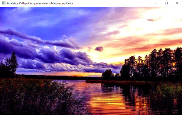
The color image will be seen as below:

Our image in color is as downloaded- i.e., it has not been manipulated in any way whatsoever. Now let us proceed to use the shape method on this image.

print(image.shape)
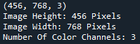
 print("Image Height: %d Pixels"%(image.shape[0]))
 print("Image Width: %d Pixels"%(image.shape[1]))
 print("Number Of Color Channels: %d "%(image.shape[2]))

Output to the above code will be seen as follows:

Notice that there is a third number present in the tuple. This is the number of color channels present in the image. The particular color channel present in this image is BGR Color Channel. It is BGR, not RGB.

Because the image is in standard color, looking at the image one can see several mixtures and shades of color. It is because there are three color channels- each element of the pixel array, has three values ranging from 0 to 255 and each value represents the intensity of BGR (Blue, Green, Red) at that particular pixel, therefore
allowing for the colors to be mixed and manipulated. We will focus more on color images in future articles.

Learning How to Resize an Image.

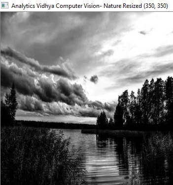
Coming back to our GRAYSCALE image, we will now attempt to resize the image, to make it cover a smaller surface area on our computer screen. To rescale an image, we need to use the resize() method offered by the OpenCV Library.

import cv2
 # load the image in a GRAYSCALE format
 image = cv2.imread("C:/Users/Shivek/Pictures/cd0c13629f217c1ab72c61d0664b3f99.jpg", cv2.IMREAD_GRAYSCALE)
 cv2.imshow('Analytics Vidhya Computer Vision- Nature Standard Image', image)
 cv2.waitKey()
 cv2.destroyAllWindows()

 # resize the image to be pixel dimensions 350 by 350
 resized_image = cv2.resize(image, dsize=(350, 350))
 cv2.imshow('Analytics Vidhya Computer Vision- Nature Resized (350, 350)', resized_image)
 cv2.waitKey()
 cv2.destroyAllWindows()

resized_image = cv2.resize(src=image, dsize=(350, 350))

We make use of the resize() method to resize the image at hand- this could mean either increasing the size or decreasing it. We chose to decrease the image size, i.e., make it smaller. This method takes in two primary arguments:

1. src = The Source Image (Image to
   be resized).
2. dsize = The Desired Size.
   It requires that you specify the pixel dimensions for height and width, between which the image will be resized. The values need to be passed in an immutable tuple. We have specified a height and width of both 350 pixels.

cv2.imshow('Analytics Vidhya Computer Vision- Nature Resized (350, 350)', resized_image)
cv2.waitKey()
cv2.destroyAllWindows()

Up to this point, one should be familiar with what the three lines of code above do- It will display the window, wait an indefinite period of time, and terminate all windows upon user command.

The last task for us would be to verify that the image size has been reduced.

The output will be seen as follows:

This concludes my article on . I do hope that you enjoyed reading through this article and have added new information to your knowledge base.

Please feel free to connect with me on LinkedIn.

Thank you for your time.

The media shown in this article are not owned by Analytics Vidhya and are used at the Author’s discretion.

Login to continue reading and enjoy expert-curated content.

Free Courses