AUC-ROC Curve in Machine Learning

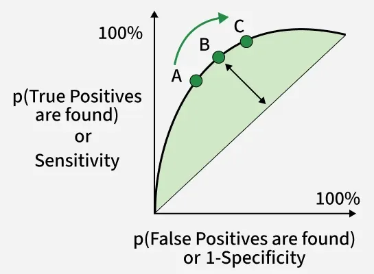
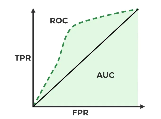
AUC-ROC curve is a graph used to check how well a binary classification model works. It helps us to understand how well the model separates the positive cases like people with a disease from the negative cases like people without the disease at different threshold level. It shows how good the model is at telling the difference between the two classes by plotting:

• True Positive Rate (TPR): How often the model correctly predicts the positive cases also known as Sensitivity or Recall.
• False Positive Rate (FPR): How often the model incorrectly predicts a negative case as positive.
• Specificity: Measures the proportion of actual negatives that the model correctly identifies. It is calculated as 1 - FPR.

A better model has a higher AUC (Area Under the Curve), which indicates a stronger ability to distinguish between classes.

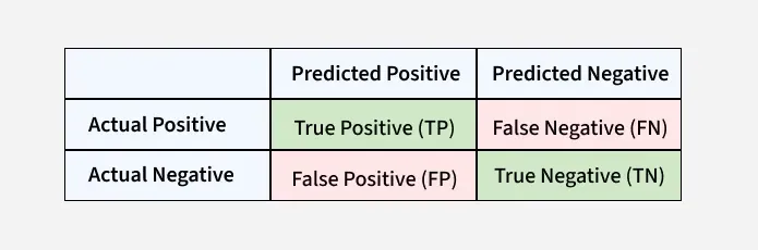
These terms are derived from the confusion matrix which provides the following values:

• True Positive (TP): Correctly predicted positive instances
• True Negative (TN): Correctly predicted negative instances
• False Positive (FP): Incorrectly predicted as positive
• False Negative (FN): Incorrectly predicted as negative

• ROC Curve : It plots TPR vs. FPR at different thresholds. It represents the trade-off between the sensitivity and specificity of a classifier.
• AUC(Area Under the Curve): measures the area under the ROC curve. A higher AUC value indicates better model performance as it suggests a greater ability to distinguish between classes. An AUC value of 1.0 indicates perfect performance while 0.5 suggests it is random guessing.

Working of AUC-ROC

AUC-ROC curve helps us understand how well a classification model distinguishes between the two classes. Imagine we have 6 data points and out of these:

• 3 belong to the positive class: Class 1 for people who have a disease.
• 3 belong to the negative class: Class 0 for people who don’t have disease.

Now the model will give each data point a predicted probability of belonging to Class 1. The AUC measures the model's ability to assign higher predicted probabilities to the positive class than to the negative class. Here’s how it work:

1. Randomly choose a pair: Pick one data point from the positive class (Class 1) and one from the negative class (Class 0).
2. Check if the positive point has a higher predicted probability: If the model assigns a higher probability to the positive data point than to the negative one for correct ranking.
3. Repeat for all pairs: We do this for all possible pairs of positive and negative examples.

When to Use AUC-ROC

AUC-ROC is effective when:

• The dataset is balanced and the model needs to be evaluated across all thresholds.
• False positives and false negatives are of similar importance.

In cases of highly imbalanced datasets AUC-ROC might give overly optimistic results. In such cases the Precision-Recall Curve is more suitable focusing on the positive class.

Model Performance with AUC-ROC:

• High AUC (close to 1): The model effectively distinguishes between positive and negative instances.
• Low AUC (close to 0): The model struggles to differentiate between the two classes.
• AUC around 0.5: The model doesn’t learn any meaningful patterns i.e it is doing random guessing.

In short AUC gives you an overall idea of how well your model is doing at sorting positives and negatives, without being affected by the threshold you set for classification. A higher AUC means your model is doing good.

Implementation using two different models

1. Installing Libraries

We will be importing numpy, pandas, matplotlib and scikit learn.

2. Generating data and splitting data

Using an 80-20 split ratio, the algorithm creates artificial binary classification data with 20 features, divides it into training and testing sets and assigns a random seed to ensure reproducibility.

3. Training the different models

To train the Random Forest and Logistic Regression models we use a fixed random seed to get the same results every time we run the code. First we train a logistic regression model using the training data. Then use the same training data and random seed we train a Random Forest model with 100 trees.

4. Predictions

Using the test data and a trained Logistic Regression model the code predicts the positive class's probability. In a similar manner, using the test data, it uses the trained Random Forest model to produce projected probabilities for the positive class.

5. Creating a dataframe

Using the test data the code creates a DataFrame called test_df with columns labeled "True," "Logistic" and "RandomForest," add true labels and predicted probabilities from Random Forest and Logistic Regression models.

6. Plotting ROC Curve for models

Plot the ROC curve and compute the AUC for both Logistic Regression and Random Forest. The ROC curve compares models based on True Positive Rate vs False Positive Rate, while the red dashed line shows random guessing.

Output:

👁 roc-Geeksforgeeks

The plot computes the AUC and ROC curve for each model i.e Random Forest and Logistic Regression, then plots the ROC curve. The ROC curve for random guessing is also represented by a red dashed line and labels, a title and a legend are set for visualization.

AUC-ROC for a Multi-Class Model

For multiclass classification, AUC-ROC is extended using the One-vs-All (OvA) approach. Each class is treated as the positive class once, and the remaining classes are grouped as the negative class. For example, if you have classes A, B, C, D, you will get four ROC curves one for each class:

• Class A vs. (B, C, D)
• Class B vs. (A, C, D)
• Class C vs. (A, B, D)
• Class D vs. (A, B, C)

Steps to Use AUC-ROC for Multiclass Models

1. One-vs-All Conversion: Treat each class as the positive class and all others combined as the negative class.

2. Train a Binary Classifier per Class: Fit the model separately for each class-vs-rest combination.

3. Compute AUC-ROC for Each Class:

• Plot the ROC curve for every class
• Calculate the AUC value for each curve

4. Compare Performance: A higher AUC score means the model is better at distinguishing that class from the others.

Implementation of AUC-ROC in Multiclass Classification

1. Importing Libraries

The program creates artificial multiclass data, divides it into training and testing sets and then uses the One-vs-Restclassifier technique to train classifiers for both Random Forest and Logistic Regression. It plots the two models multiclass ROC curves to demonstrate how well they discriminate between various classes.

2. Generating Data and splitting

Three classes and twenty features make up the synthetic multiclass data produced by the code. After label binarization, the data is divided into training and testing sets in an 80-20 ratio.

3. Training Models

The program trains two multiclass models i.e a Random Forest model with 100 estimators and a Logistic Regression model with the One-vs-Rest approach. With the training set of data both models are fitted.

4. Plotting the AUC-ROC Curve

The ROC curves and AUC scores for each class are computed and plotted for both models. A dashed line indicates random guessing, helping visualize how well each model separates multiple classes.

Output:

👁 multi-Geeksforgeeks

• The Random Forest and Logistic Regression models ROC curves and AUC scores are calculated by the code for each class.
• The multiclass ROC curves are then plotted showing the discrimination performance of each class and featuring a line that represents random guessing.
• The resulting plot offers a graphic evaluation of the models' classification performance.