Gaussian Mixture Model (GMM) is a probabilistic clustering technique that models data as a combination of multiple Gaussian distributions, allowing more flexible grouping of data points.
Assigns each data point a probability of belonging to different clusters
Can handle overlapping clusters effectively
Uses mean and covariance to define cluster shape
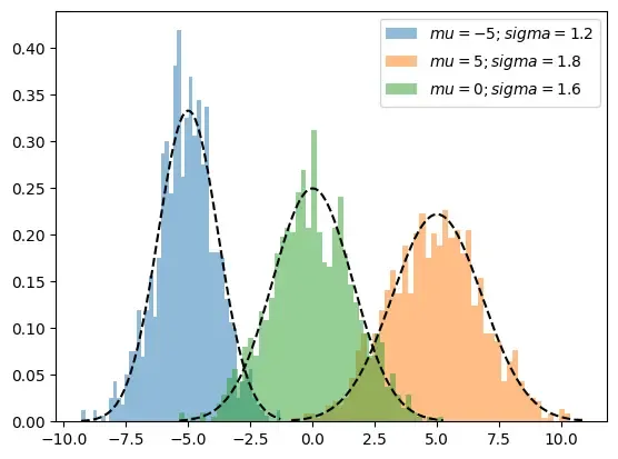
👁 GMM Visualization of three distinct one-dimensional Gaussian distributions
The above shown graph shows a three one-dimensional Gaussian distributions with distinct means and variances. Each curve represents the theoretical probability density function (PDF) of a normal distribution, highlighting differences in location and spread.
A Gaussian Mixture Model assumes that the data is generated from a mixture of K Gaussian distributions, each representing a cluster. Every Gaussian has its own mean , covariance and mixing weight .
1. Posterior Probability (Cluster Responsibility)
For a given data point xn, the probability that it belongs to cluster k:
where:
is a latent variable indicating cluster assignment
is the mixing probability of the k-th Gaussian.
is the Gaussian distribution with mean and covariance
2. Likelihood of a Data Point
The total likelihood of observing xnx_nxn under all Gaussians is:
This represents how well the mixture as a whole explains the data point.
3. Expectation-Maximization (EM) Algorithm
GMM parameters are estimated using the EM algorithm:
E-step (Expectation): Compute the responsibility of each cluster for every data point using current parameter values.
M-step (Maximization): Update
Means
Covariances
Mixing coefficients using the responsibilities from the E-step. The process continues until the model's log-likelihood stabilizes.
4. Log-Likelihood of the Mixture Model
The objective optimized by EM is:
EM increases this likelihood in every iteration.
Cluster Shapes in GMM
In GMM, each cluster is a Gaussian defined by:
Mean (μ): Center of the cluster.
Covariance (Σ): Controls the shape, orientation and spread of the cluster.
Because covariance matrices allow elliptical shapes, GMM can model:
elongated clusters
tilted clusters
overlapping clusters
This makes GMM more flexible than methods like K-Means, which assumes only spherical clusters.
Visualizing GMM often involves:
Scatter plots showing raw data
Elliptical contours (or KDE curves) showing the shape of each Gaussian component
These illustrate how GMM adapts to complex, real-world data distributions.
Implementing Gaussian Mixture Model (GMM)
Import required libraries. make_blobs creates a simple synthetic dataset for demo.
Step 1: Generate synthetic data
creates 500 points in 2D grouped around 3 centers. cluster_std controls how tight or spread each cluster is. y is the true label (only for reference).
Step 2: Fit the Gaussian Mixture Model
fit(X) runs the EM algorithm to learn means, covariances and mixing weights.
labels gives the cluster index for each point (the component with highest posterior probability).
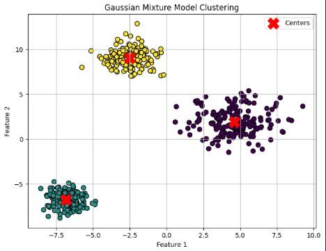
Step 3: Plot clusters and component centers
Points colored by assigned cluster and red X marks showing the learned Gaussian centers.
