Support Vector Regression (SVR) using Linear and Non-Linear Kernels in Scikit Learn

Support Vector Regression predicts continuous values by fitting a function within a defined error margin. It uses kernel functions to handle both linear relationships and complex non-linear patterns in data.

• Works well with high-dimensional data
• Uses linear and kernel-based transformations
• Controls model flexibility using regularization parameters
• Effective for real-world datasets with limited samples

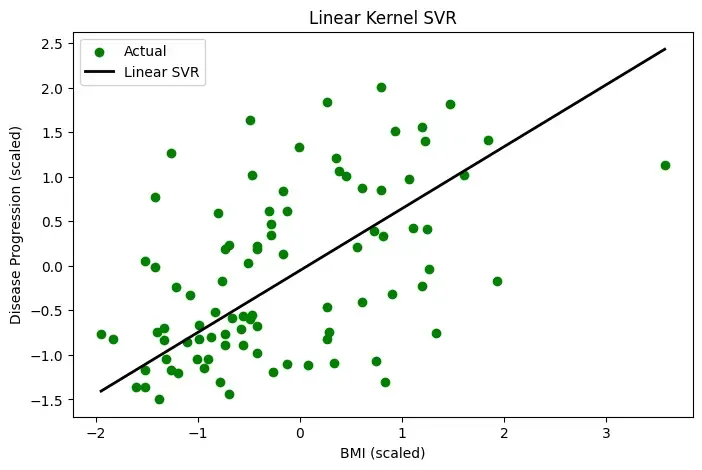
Linear Kernel SVR

Linear SVR is used when the relationship between input features and the target variable is approximately linear. It fits a straight regression function in the original feature space without transforming the data into higher dimensions.

Kernel Function:

When to use

• Data shows a linear trend
• Large datasets with many features
• Interpretability is important

Linear SVR is computationally efficient, interpretable and suitable for datasets where features have a direct and proportional relationship with the output.

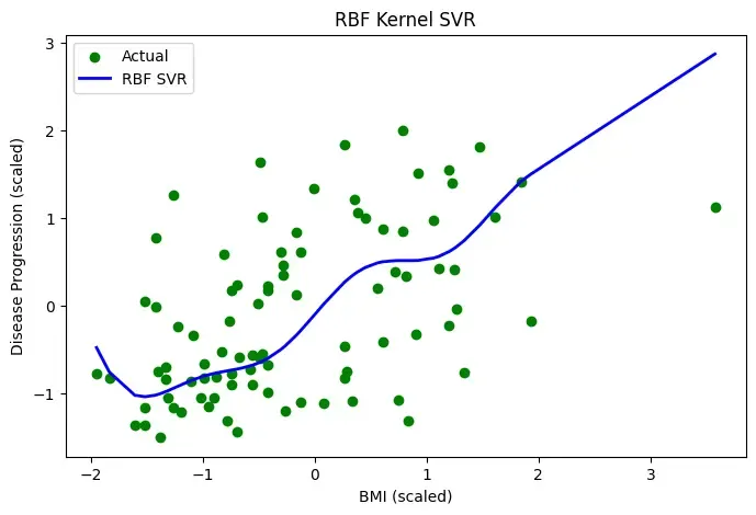
Non-Linear Kernel SVR

Non-linear SVR is applied when the relationship between input and output is complex and cannot be captured by a straight line. It uses kernel functions to implicitly map data into higher-dimensional spaces where a linear relationship can be learned.

This enables SVR to model curved patterns and complex feature interactions commonly found in real-world data.

Common Non-Linear Kernels

• RBF (Gaussian) Kernel: The RBF kernel is the most widely used non-linear kernel in SVR. It measures similarity based on distance and allows the model to create smooth, flexible regression curves. It is highly effective for capturing localized and non-linear patterns.
• Polynomial Kernel: The polynomial kernel models polynomial relationships between features and targets. It is useful when interactions between features follow polynomial behaviour but can become computationally expensive for higher degrees.
• Sigmoid Kernel: The sigmoid kernel resembles neural network activation functions and is less commonly used in regression tasks due to stability issues.

Implementation

Let's see a step-by-step SVR implementation.

Step 1: Import Libraries

We need to import the necessary libraries such a NumPy, Matplotlib, sklearn,

Step 2: Load Dataset

Here:

• The diabetes dataset is loaded directly from Scikit-Learn
• X contains medical input features
• y contains disease progression values

Step 3: Select One Feature

Here:

• Only the BMI feature is selected from the dataset
• Data is reshaped into a 2D array as required by Scikit-Learn
• Simplifies visualization to a 1D regression curve

Step 4: Train-Test Split

Dataset is split into training and testing subsets, 80% data is used for training and 20% for testing.

Step 5: Feature Scaling

• Separate scalers are created for input features and target values
• Training data is standardized to zero mean and unit variance
• Test data is transformed using the same scaling parameters
• Target values are also scaled for stable SVR optimization

Step 6: Train Linear Kernel SVR

Here:

• A Linear SVR model is created
• C=100 controls error penalty strength
• epsilon=0.1 defines the tolerance margin
• Model learns a straight regression function
• Predictions are generated on test data

Step 7: Train RBF Kernel SVR

• An RBF (non-linear) SVR model is created
• gamma controls influence range of data points
• Model learns a smooth, non-linear regression curve
• Predictions are generated for comparison

Step 8: Sort Test Data

• Test input values are sorted in ascending order
• Corresponding actual and predicted values are reordered

Step 9: Plot Linear SVR

Here we plot the linear SVR:

Output:

Step 10: Plot RBF SVR

We plot the RBF SVR:

Output:

Step 11: Evaluate Models

a. Linear SVR

• RMSE measures average prediction error magnitude
• MAE measures absolute deviation from actual values
• Higher values indicate weaker performance

Output:

Linear SVR RMSE: 0.8423305650413904
Linear SVR MAE: 0.6735880994376383

b. RBF SVR

• Same metrics are computed for fair comparison
• Lower RMSE and MAE indicate better model fit
• Confirms numerical superiority of Linear SVR for this dataset

Output:

RBF SVR RMSE: 0.8753416035431131
RBF SVR MAE: 0.6797975426553673

Applications

• Medical Prediction: Used to estimate disease progression and patient health outcomes from clinical data.
• Financial Forecasting: Applied in predicting stock prices, returns and market trends with non-linear behavior.
• Energy Demand Estimation: Helps forecast electricity load and energy consumption patterns.
• Sales Forecasting: Used to predict product demand and future sales in business analytics.
• Engineering Modelling: Applied in modeling physical systems and scientific regression problems.

Advantages

• Good Generalization: Margin-based learning helps SVR perform well on unseen data.
• Handles Non-Linearity: Kernel functions allow SVR to model complex relationships.
• Robust to Noise: ε-insensitive loss reduces sensitivity to small errors and noise.
• Effective with Small Data: Performs well even with limited training samples.
• Kernel Flexibility: Different kernels can be chosen based on problem requirements.

Limitations

• Hyperparameter Sensitivity: Requires careful tuning of C, ε and kernel parameters.
• High Computational Cost: Training becomes slow for large datasets.
• Scaling Requirement: Feature scaling is mandatory for good performance.
• Low Interpretability: Non-linear SVR models are hard to interpret.
• Kernel Selection Difficulty: Choosing the right kernel often needs experimentation.