Affinity Propagation

Affinity Propagation (AP) is a clustering algorithm that automatically identifies clusters and their exemplars (representative points) without requiring you to specify the number of clusters in advance. Unlike methods such as K-Means, Affinity Propagation determines cluster centers by iteratively exchanging “messages” between data points to identify the most suitable exemplars.

Suppose a dataset of fruits with features like color, size and weight. Affinity Propagation can group similar fruits:

• Apples with apples
• Bananas with bananas

Note: The algorithm does not require prior labels, it clusters purely based on similarity.

Working

1. Similarity Computation

It starts with a similarity matrix s, where S(i,j) represents the similarity between points x_i and x_j .

By default, similarity is calculated as negative squared Euclidean distance:

Diagonal elements S(i,i) are called preferences, indicating how likely each point is to be chosen as an exemplar. A higher preference is more likely to become a cluster centre.

2. Responsibility Update

The responsibility matrix reflects how suitable a point is to be the exemplar for point , relative to other candidates:

A high means is much more suitable than any other candidate to represent .

3. Availability Update

The availability matrix represents how appropriate it is for to choose as its exemplar, considering the preferences of other points:

For :

For (self-availability):

Responsibility reflects a candidate’s suitability; availability reflects the support from other points.

4. Iterative Updates and Convergence

and are updated iteratively until convergence.

Exemplars are points where:

Each point is then assigned to its nearest exemplar, forming clusters.

Visualizing the Process

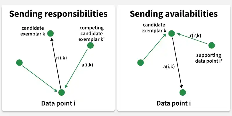
In Affinity Propagation, messages are passed between data points in two main steps:

Responsibility (Left Side): These messages shows how each data point communicates with its candidate exemplars. Each point sends responsibility messages to suggest how suitable it is to be chosen as an exemplar.

Availability (Right Side): These messages reflect how appropriate it is for each data point to choose its corresponding exemplar considering the support from other points. Essentially, these messages show how much support the candidate exemplars have.

Key Parameters Influencing Clustering

There are mainly two parameters that influence the process of clustering.

1. Preference

• Controls the number of exemplars (cluster centers).
• Higher preference → more exemplars → more clusters.
• Lower preference → fewer exemplars → fewer clusters.
• Choosing the right preference is important to balance under and over-clustering.

2. Damping Factor

• Helps stabilize the algorithm by limiting the update size between iterations.
• Without damping, the algorithm may oscillate or fail to converge.
• Typical values are between 0.5 and 1.0, with higher values slowing convergence but increasing stability.

Step-by-step implementation

Here we will see its step by step working:

1. Importing required libraries

At first we will import all required Python libraries like NumPy, Matplotlib, Seaborn, Pandas and Scikit learn.

2. Dataset loading and Pre-Processing

Now we load the dataset for clustering. After that we will use to Standard Scaler to prepare the dataset for Affinity propagation.

You can download the dataset from here.

3. Exploratory Data Analysis

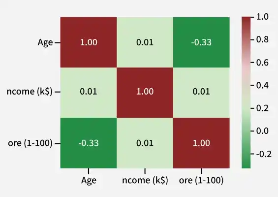
Exploratory Data Analysis (EDA) helps us to gain deeper insights about the dataset which is very important in clustering algorithm implementation.Visualizing correlation matrix will help us to understand how the features are correlated to each other.

Output:

So from it we can see that we can only select these three features. And as you can see we have only selected two features in our code of Data loading subsection.

4. Pairwise Feature Scatter Plots

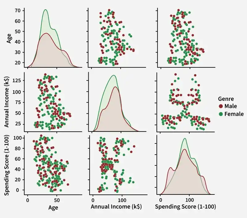
This plot grid shows scatter plots and histograms for every pair of features. It helps us understand feature distribution, relationships between variables and overall data patterns in a single view.

Output:

5. Affinity Propagation Clustering and Performance Evaluation

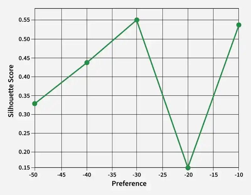
We now apply Affinity Propagation by setting its key parameters:

• preference: Controls how likely a point is to become an exemplar and affects the number of clusters.
• max_iter: Maximum number of iterations allowed.
• convergence_iter: Number of stable iterations needed before the algorithm stops.
• random_state: Ensures consistent results across runs.
• damping: Slows updates to avoid oscillation; a value like 0.9 increases stability but slows convergence.

Output:

Here -30 resulting in higher value of preference parameter is the optimal preference.

6. Applying Affinity Propagation Clustering

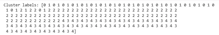
We will apply Affinity Propagation to group the data points into clusters.

Output:

7. Evaluating its Performance

We will evaluate its performance using Silhouette Score.

Output:

Silhouette Score: 0.5529643053885619

Silhouette Score of 0.5529 represents a reasonably good degree of separation between the clusters. TA silhouette score > 0 indicates some separation between clusters, but not necessarily no overlap. Values closer to 1 represent better clustering.

8. Visualizing Clusters

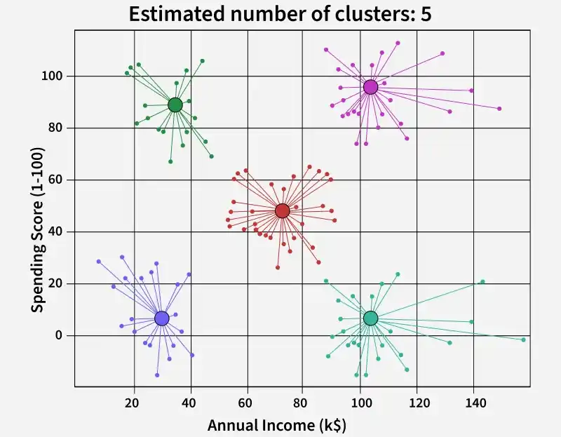
We will create a plot where clustering effect can be visualized.

Output:

Applying Affinity Propagation resulted in 5 distinct and well-separated clusters, clearly segmenting the customers based on their income and spending scores

You can download the complete code from here .

Benefits

1. Automatic cluster detection: Finds both number of clusters and centers without pre-specifying them.
2. Robust to noise and outliers: Works well even with noisy data.
3. Handles non-spherical clusters: Unlike K-Means, AP is not restricted to spherical clusters.
4. Scalability: Suitable for moderately large datasets, but requires O(n²) memory for the similarity matrix.

Applications

• Image and Video Analysis: Used for object recognition, image segmentation and video summarization by grouping similar regions or objects.
• Natural Language Processing: Helps in document clustering, topic grouping and sentiment analysis by identifying similar text patterns.
• Bioinformatics: Applied to gene expression data, protein structure grouping and interaction network clustering to find meaningful biological patterns.
• Social Network Analysis: Identifies communities in networks by clustering users based on their connections.
• Market Segmentation: Groups customers by behavior, preferences or demographics to support targeted marketing.