KMeans Clustering and PCA on Wine Dataset

K-Means Clustering: K Means Clustering is an unsupervised learning algorithm that tries to cluster data based on their similarity. Unsupervised learning means that there is no outcome to be predicted, and the algorithm just tries to find patterns in the data. In k means clustering, we specify the number of clusters we want the data to be grouped into. The algorithm randomly assigns each observation to a set and finds the centroid of each set. Then, the algorithm iterates through two steps: Reassign data points to the cluster whose centroid is closest. Calculate the new centroid of each cluster. These two steps are repeated until the within-cluster variation cannot be reduced further. The within-cluster deviation is calculated as the sum of the Euclidean distance between the data points and their respective cluster centroids.

In this article, we will cluster the wine datasets and visualize them after dimensionality reductions with PCA.

Importing libraries needed for dataset analysis

We will first import some useful Python libraries like Pandas, Seaborn, Matplotlib and SKlearn for performing complex computational tasks. 

 Importing Dataset:

These data are the results of a chemical analysis of wines grown in the same region in Italy but derived from three different cultivars. The analysis determined the quantities of 13 constituents found in each of the three types of wines

Output :

	alcohol	malic_acid	ash	alcalinity_of_ash	magnesium	total_phenols	flavanoids	nonflavanoid_phenols	proanthocyanins	color_intensity	hue	od280/od315_of_diluted_wines	proline	target
0	14.23	1.71	2.43	15.6	127.0	2.80	3.06	0.28	2.29	5.64	1.04	3.92	1065.0	0
1	13.20	1.78	2.14	11.2	100.0	2.65	2.76	0.26	1.28	4.38	1.05	3.40	1050.0	0
2	13.16	2.36	2.67	18.6	101.0	2.80	3.24	0.30	2.81	5.68	1.03	3.17	1185.0	0
3	14.37	1.95	2.50	16.8	113.0	3.85	3.49	0.24	2.18	7.80	0.86	3.45	1480.0	0
4	13.24	2.59	2.87	21.0	118.0	2.80	2.69	0.39	1.82	4.32	1.04	2.93	735.0	0

Because We are doing here the unsupervised learning. So we remove the target Customer_Segment column from our datasets.

Output:

<class 'pandas.core.frame.DataFrame'>
RangeIndex: 178 entries, 0 to 177
Data columns (total 13 columns):
 # Column Non-Null Count Dtype 
--- ------ -------------- ----- 
 0 alcohol 178 non-null float64
 1 malic_acid 178 non-null float64
 2 ash 178 non-null float64
 3 alcalinity_of_ash 178 non-null float64
 4 magnesium 178 non-null float64
 5 total_phenols 178 non-null float64
 6 flavanoids 178 non-null float64
 7 nonflavanoid_phenols 178 non-null float64
 8 proanthocyanins 178 non-null float64
 9 color_intensity 178 non-null float64
 10 hue 178 non-null float64
 11 od280/od315_of_diluted_wines 178 non-null float64
 12 proline 178 non-null float64
dtypes: float64(13)
memory usage: 18.2 KB

Scaling the Data:

Data is scaled using StandardScaler except for the target column(Customer_Segment), whose values must remain unchanged.

Output:

	alcohol	malic_acid	ash	alcalinity_of_ash	magnesium	total_phenols	flavanoids	nonflavanoid_phenols	proanthocyanins	color_intensity	hue	od280/od315_of_diluted_wines	proline
0	1.518613	-0.562250	0.232053	-1.169593	1.913905	0.808997	1.034819	-0.659563	1.224884	0.251717	0.362177	1.847920	1.013009
1	0.246290	-0.499413	-0.827996	-2.490847	0.018145	0.568648	0.733629	-0.820719	-0.544721	-0.293321	0.406051	1.113449	0.965242

In general, K-Means requires unlabeled data in order to run. 

So, taking data without labels to perform K-means clustering.

Elbow Method

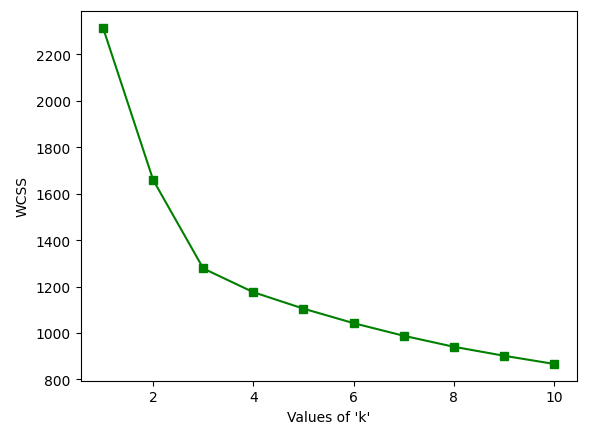
The elbow Method is used to determine the number of clusters

Output:

👁 Elbow Curve -Geeksforgeeks

As we can see from the above graph that there is turning like an elbow at k=3. So, we can say that the right number of cluster for the given datasets is 3.

Implementing K-Means:

Let's perform the K-Means clustering for n_clusters=3.

Output :

KMeans(n_clusters=3)

For each cluster, there are values of cluster centers according to the number of columns present in the data.

Output :

array([[ 0.83523208, -0.30380968, 0.36470604, -0.61019129, 0.5775868 ,
 0.88523736, 0.97781956, -0.56208965, 0.58028658, 0.17106348,
 0.47398365, 0.77924711, 1.12518529],
 [-0.92607185, -0.39404154, -0.49451676, 0.17060184, -0.49171185,
 -0.07598265, 0.02081257, -0.03353357, 0.0582655 , -0.90191402,
 0.46180361, 0.27076419, -0.75384618],
 [ 0.16490746, 0.87154706, 0.18689833, 0.52436746, -0.07547277,
 -0.97933029, -1.21524764, 0.72606354, -0.77970639, 0.94153874,
 -1.16478865, -1.29241163, -0.40708796]])

labels_ Index of the cluster each sample belongs to.

Output :

array([0, 0, 0, 0, 0, 0, 0, 0, 0, 0, 0, 0, 0, 0, 0, 0, 0, 0, 0, 0, 0, 0,
 0, 0, 0, 0, 0, 0, 0, 0, 0, 0, 0, 0, 0, 0, 0, 0, 0, 0, 0, 0, 0, 0,
 0, 0, 0, 0, 0, 0, 0, 0, 0, 0, 0, 0, 0, 0, 0, 1, 1, 2, 1, 1, 1, 1,
 1, 1, 1, 1, 1, 1, 1, 0, 1, 1, 1, 1, 1, 1, 1, 1, 1, 2, 1, 1, 1, 1,
 1, 1, 1, 1, 1, 1, 1, 0, 1, 1, 1, 1, 1, 1, 1, 1, 1, 1, 1, 1, 1, 1,
 1, 1, 1, 1, 1, 1, 1, 1, 2, 1, 1, 0, 1, 1, 1, 1, 1, 1, 1, 1, 2, 2,
 2, 2, 2, 2, 2, 2, 2, 2, 2, 2, 2, 2, 2, 2, 2, 2, 2, 2, 2, 2, 2, 2,
 2, 2, 2, 2, 2, 2, 2, 2, 2, 2, 2, 2, 2, 2, 2, 2, 2, 2, 2, 2, 2, 2,
 2, 2], dtype=int32)

Apply Dimensionality Reduction Technique PCA

Principal Component Analysis is a technique that transforms high-dimensions data into lower-dimension while retaining as much information as possible.

• It is used to interpret and visualize data. 
• The number of variables decreases, which simplifies further analysis.

We can then view the PCA components_, i.e. the principal axes in the feature space, which represent the directions of maximum variance in the dataset. These components are sorted by explained_variance_.

Minimize the dataset from 15 features to 2 features using principal component analysis (PCA).

Output :

	PCA1	PCA2
0	3.316751	-1.443463
1	2.209465	0.333393
2	2.516740	-1.031151
3	3.757066	-2.756372
4	1.008908	-0.869831

Reducing centers:

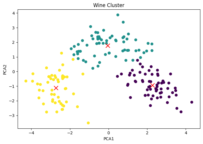
Reducing the cluster centers using PCA.

Output :

array([[ 2.2761936 , -0.93205403],
 [-0.03695661, 1.77223945],
 [-2.72003575, -1.12565126]])

Represent the cluster plot based on PCA1 and PCA2. Differentiate clusters by passing a color parameter as c=kmeans.labels_

Output :

👁 Wine Cluster

Effect of PCA1 & PCA2 on Clusters:

If we really want to reduce the size of the dataset, the best number of principal components is much less than the number of variables in the original dataset.

Output :

array([[ 0.1443294 , -0.24518758, -0.00205106, -0.23932041, 0.14199204,
 0.39466085, 0.4229343 , -0.2985331 , 0.31342949, -0.0886167 ,
 0.29671456, 0.37616741, 0.28675223],
 [-0.48365155, -0.22493093, -0.31606881, 0.0105905 , -0.299634 ,
 -0.06503951, 0.00335981, -0.02877949, -0.03930172, -0.52999567,
 0.27923515, 0.16449619, -0.36490283]])

Represent the effect Features on PCA components.

Output :

👁 Effect of each features on PCA 1 and PCA2 -Geeksforgeeks