Precision-Recall Curve - ML

Precision-Recall Curve (PR Curve) is a graphical representation that helps us understand how well a binary classification model is doing especially when the data is imbalanced which means when one class is more dominant than other. In this curve:

• x-axis shows recall also called sensitivity or true positive rate which tells us how many actual positive cases the model correctly identified.
• y-axis shows precision which tells us how many of the predicted positive cases were actually correct.

Unlike theROC curve which looks at both positives and negatives the PR curve focuses only on how well the model handles the positive class. This makes it useful when the goal is to detect important cases like fraud, diseases or spam messages.

Key Concepts of Precision and Recall

Before understanding the PR curve let’s understand:

1. Precision

It refers to the proportion of correct positive predictions (True Positives) out of all the positive predictions made by the model i.e True Positives + False Positives. It is a measure of the accuracy of the positive predictions. The formula for Precision is:

A high Precision means that the model makes few False Positives. This metric is especially useful when the cost of false positives is high such as email spam detection.

2. Recall

It is also known as Sensitivity or True Positive Rate where we measures the proportion of actual positive instances that were correctly identified by the model. It is the ratio of True Positives to the total actual positives i.e True Positives + False Negatives. The formula for Recall is:

A high Recall means the model correctly identifies most of the positive instances which is critical when False Negatives are costly like in medical diagnoses.

3. Confusion Matrix

To better understand Precision and Recall we can use a Confusion Matrix which summarizes the performance of a classifier in four essential terms:

• True Positives (TP): Correctly predicted positive instances.
• False Positives (FP): Incorrectly predicted positive instances.
• True Negatives (TN): Correctly predicted negative instances.
• False Negatives (FN): Incorrectly predicted negative instances.

How Precision-Recall Curve Works

The PR curve is created by changing the decision threshold of your model and checking how the precision and recall change at each step. The threshold is the cutoff point where you decide:

• If the probability is above the threshold you predict positive.
• If it's below you predict negative.

By default this threshold is usually 0.5 but you can move it up or down.

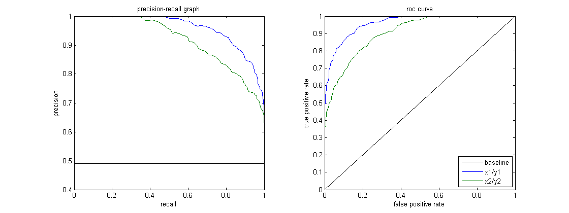
A PR curve is useful when dealing with imbalanced datasets where one class significantly outnumbers the other. In such cases the ROC curve might show overly optimistic results as it doesn’t account for class imbalance as effectively as the Precision-Recall curve. The figure below shows a comparison of sample PR and ROC curves. It is desired that the algorithm should have both high precision and high recall. However most machine learning algorithms often involve a trade-off between the two. A good PR curve has greater AUC (area under the curve).

In the figure above the classifier corresponding to the blue line has better performance than the classifier corresponding to the green line. It is important to note that the classifier that has a higher AUC on the ROC curve will always have a higher AUC on the PR curve as well.

Interpreting a Precision-Recall Curve

Consider an algorithm that classifies whether or not a document belongs to the category "Sports" news. Assume there are 12 documents with the following ground truth (actual) and classifier output class labels.

Now let us find TP, TN, FP and FN values.

• True Positives (TP): Documents that were accurately categorised as "Sports" and that were in fact about sports. Documents D1, D2, D10 and D11 in this scenario are instances of TP.
• True Negatives (TN): True Negatives are those cases in which the document was appropriately labelled as "Not sports" even though it had nothing to do with sports. In this instance TN is demonstrated by documents D5, D8 and D9.
• False Positives (FP): Documents that were mistakenly categorised as "Sports" even though they had nothing to do with sports. Here are some FP examples documents D3 and D7.
• False Negatives (FN): Examples of documents that were mistakenly labelled as "Not sports" but in reality they were about sports. Documents D4, D6 and D12 in this case are FN examples.

Given these counts: TP=4,TN=3,FP=2,FN=3

Finally precision and recall are calculated as follows:

It follows that the recall is 4/7 when the precision is 2/3. All the cases that were anticipated to be positive, two-thirds were accurately classified (precision) and of all the instances that were actually positive, the model was able to capture four-sevenths of them (recall).

When to use PR curve and ROC curve

Choosing between ROC and Precision-Recall depends on the specific needs of the problem, understanding data distribution and the consequences of different types of errors.

• The PR curve helps us visualize how well our model is performing across various thresholds. It provides insights into how changes in decision thresholds affect Precision and Recall. For example increasing the threshold might increase Precision i.e fewer False Positives but it could lower Recall i.e more False Negatives. The goal is to find a balance that best suits the specific needs of your application whether it’s minimizing False Positives or False Negatives.
• ROC curves are suitable when the class distribution is balanced and false positives and false negatives have similar consequences. They show the trade-off between sensitivity and specificity.

Implementation of Precision-Recall Curve

Step 1: Importing Necessary Libraries

We will generate precision-recall curve with scikit-learn and visualize the results with Matplotlib.

Step 2: Dataset Used

This code generates a synthetic dataset for a binary classification problem using scikit-learn's make_classification function.

Step 3: Train and Test Split

The train_test_split function in scikit-learn is used to split dataset into training and testing sets.

Step 4: Model Building

Here we are using Logistic Regression to train the model on the training data set. A popular algorithm for binary classification. It is implemented by the scikit-learn class LogisticRegression.

Step 5: Model Prediction

We will calculate Precision and Recall which will be used to draw a precision-recall curve and then we will calculate AUC for the precision-recall curve.

Step 6: Plotting PR Curve

It visualizes the precision-recall curve and evaluate the precision vs recall trade-off at various decision thresholds.

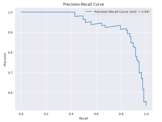
Output:

This curve shows the trade-off between Precision and Recall across different decision thresholds. The Area Under the Curve (AUC) is 0.94 suggesting that the model performs well in balancing both Precision and Recall. A higher AUC typically indicates better model performance.