Implementation of Polynomial Regression

Polynomial Regression is a form of linear regression where the relationship between the independent variable (x) and the dependent variable (y) is modelled as an degree polynomial. It is useful when the data exhibits a non-linear relationship allowing the model to fit a curve to the data.

Need for Polynomial Regression

• Non-linear Relationships: Polynomial regression is used when the relationship between the independent variable (input) and dependent variable (output) is non-linear. Unlike linear regression which fits a straight line, it fits a polynomial equation to capture the curve in the data.
• Better Fit for Curved Data: When a researcher hypothesizes a curvilinear relationship, polynomial terms are added to the model. A linear model often results in residuals with noticeable patterns which shows a poor fit. It can capture these non-linear patterns effectively.
• Flexibility and Complexity: It does not assume all independent variables are independent. By introducing higher-degree terms, it allows for more flexibility and can model more complex, curvilinear relationships between variables.

How does a Polynomial Regression work?

Polynomial regression is an extension of linear regression where higher-degree terms are added to model non-linear relationships. The general form of the equation for a polynomial regression of degree is:

where:

• is the dependent variable.
• is the independent variable.
• ​ are the coefficients of the polynomial terms.
• is the degree of the polynomial.
• represents the error term.

The goal of regression analysis is to model the expected value of a dependent variable in terms of an independent variable . In simple linear regression, this relationship is modeled as:

Here

• is a dependent variable
• is the y-intercept, is the slope
• is the error term

However in cases where the relationship between the variables is nonlinear such as modelling chemical synthesis based on temperature, a linear model may not be sufficient. Instead, we use polynomial regression which introduces higher-degree terms such as to better capture the relationship.

For example, a quadratic model can be written as:

Here:

• is the dependent variable on
• is the y-intercept and is the error rate.

In general, polynomial regression can be extended to the nth degree:

While the regression function is linear in terms of the unknown coefficients , the model itself captures non-linear patterns in the data. The coefficients are estimated using techniques like Least Square technique to minimize the error between predicted and actual values.

Choosing the right polynomial degree is important: a higher degree may fit the data more closely but it can lead to overfitting. The degree should be selected based on the complexity of the data. Once the model is trained, it can be used to make predictions on new data, capturing non-linear relationships and providing a more accurate model for real-world applications.

Real-Life Example for Polynomial Regression

Let’s consider an example in the field of finance where we analyze the relationship between an employee's years of experience and their corresponding salary. If we check that the relationship might not be linear, polynomial regression can be used to model it more accurately.

Example Data:

Now, let's apply polynomial regression to model the relationship between years of experience and salary. We'll use a quadratic polynomial (degree 2) which includes both linear and quadratic terms for better fit. The quadratic polynomial regression equation is:

To find the coefficients that minimize the difference between the predicted and actual salaries, we can use the Least Squares method. The objective is to minimize the sum of squared differences between the predicted salaries and the actual data points which allows us to fit a model that captures the non-linear progression of salary with respect to experience.

Implementation of Polynomial Regression

Here we will see how to implement polynomial regression using Python.

Step 1: Importing Required Libraries

We'll using Pandas, NumPy, Matplotlib and Sckit-Learn libraries and a random dataset for the analysis of Polynomial Regression which you can download from here.

Step 2: Loading and Preparing the Data

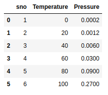
Here we will load the dataset and print it for our understanding.

Output:

Step 3: Defining Feature and Target Variables

Our feature variable that is X will contain the Column between 1^st and the target variable that is y will contain the 2^nd column. 

Step 4: Fitting the Linear Regression Model

We will first fit a simple linear regression model to the data.

Output:

Step 5: Fitting the Polynomial Regression Model

Now we will apply polynomial regression by adding polynomial terms to the feature space. In this example, we use a polynomial of degree 4.

Step 6: Visualizing the Linear Regression Results

Visualize the results of the linear regression model by plotting the data points and the regression line.

Output:

A scatter plot of the feature and target variable with the linear regression line fitted to the data.

Step 7: Visualize the Polynomial Regression Results

Now visualize the polynomial regression results by plotting the data points and the polynomial curve.

Output:

A scatter plot of the feature and target variable with the polynomial regression curve fitted to the data.

Step 8: Predict New Results

To predict new values using both linear and polynomial regression we need to ensure the input variable is in a 2D array format.

Output:

array([0.20675333])

Output:

array([0.43295877])

Balancing Overfitting and Underfitting in Polynomial Regression

In polynomial regression, overfitting happens when the model is too complex and fits the training data too closely helps in making it perform poorly on new data. To avoid this, we use techniques like Lasso and Ridge regression which helps to simplify the model by limiting the size of the coefficients.

On the other hand, underfitting occurs when the model is too simple to capture the real patterns in the data. This usually happens with a low-degree polynomial. The key is to choose the right polynomial degree to ensure the model is neither too complex nor too simple which helps it work well on both the training data and new data.

Bias Vs Variance Tradeoff

Bias Vs Variance Tradeoff helps us avoid both overfitting and underfitting by selecting the appropriate polynomial degree. As we increase the polynomial degree, the model fits the training data better but after a certain point, it starts to overfit. This is visible when the gap between training and validation errors begins to widen. The goal is to choose a polynomial degree where the model captures the data patterns without becoming too complex which ensures a good generalization.

Application of Polynomial Regression

1. Modeling Growth Rates: Polynomial regression is used to model non-linear growth rates such as the growth of tissues over time.
2. Disease Epidemic Progression: It helps track and predict the progression of disease outbreaks, capturing the non-linear nature of epidemic curves.
3. Environmental Studies: It is applied in studies like the distribution of carbon isotopes in lake sediments where relationships are non-linear.
4. Economics and Finance: It is used to analyze non-linear relationships in financial markets, predicting trends and fluctuations over time.

Advantages

1. Fits a Wide Range of Curves: Polynomial regression can model a broad range of non-linear relationships helps in making it versatile for complex data.
2. Captures Non-linear Patterns: It provides a more accurate approximation of relationships when data follows a curvilinear pattern, unlike linear regression.
3. Flexible Modeling: It can capture and represent the nuances in the data helps in making it ideal for situations where linear models fail.

Disadvantages

1. Sensitivity to Outliers: It is highly sensitive to outliers and a few extreme values can skew the results significantly.
2. Overfitting: With higher-degree polynomials, there’s a risk of overfitting where the model becomes too complex and fails to generalize well to new data.
3. Limited Outlier Detection: Unlike linear regression, it has fewer built-in methods for detecting or handling outliers helps in making it challenging to identify when the model is affected by them.

By mastering polynomial regression, we can better model complex data patterns which leads to more accurate predictions and valuable insights across various fields.