QR Decomposition in Machine learning

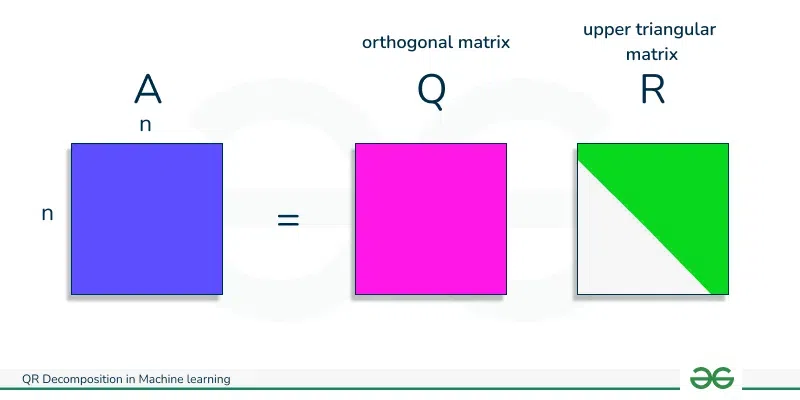
QR decomposition is a way of expressing a matrix as the product of two matrices: Q (an orthogonal matrix) and R (an upper triangular matrix). In this article, I will explain decomposition in Linear Algebra, particularly QR decomposition among many decompositions.

What is QR Decomposition?

Decomposition or Factorization is dividing the original single entity into multiple entities for easiness. Decomposition has various applications in numerical linear algebra, optimization, solving systems of linear equations, etc. QR decomposition is a versatile tool in numerical linear algebra that finds applications in solving linear systems, least squares problems, eigenvalue computations, etc. Its numerical stability and efficiency make it a valuable technique in a range of applications.

QR decomposition, also known as QR factorization, is a fundamental matrix decomposition technique in linear algebra. QR decomposition is a matrix factorization technique that decomposes a matrix into the product of an orthogonal matrix (Q) and an upper triangular matrix (R). Given a matrix A (m x n), where m is the number of rows and n is the number of columns, the QR decomposition can be expressed as:

👁 QR Decomposition in Machine learning

QR decomposition finds widespread use in machine learning for tasks like solving linear regression, eigenvalue problems, Gram-Schmidt orthogonalization, handling overdetermined systems, matrix inversion, Gram matrix factorization, and enhancing numerical stability in various algorithms. More details about it, is in the application section.

QR Decomposition Related Concepts

1. Matrix Factorization: Matrix factorization involves expressing a matrix as the product of two or more matrices. In QR decomposition, we express a given matrix A as the product of an orthogonal matrix Q and an upper triangular matrix R.
2. Orthogonal Matrix: An orthogonal matrix Q has the property that its transpose is equal to its inverse (Q^T * Q = I, where I is the identity matrix).
   • Properties: Orthogonal matrices preserve the length of vectors and the dot product. They play a crucial role in QR decomposition.
3. Upper Triangular Matrix: A matrix is upper triangular if all entries below the main diagonal are zero. In QR decomposition, R is an upper triangular matrix.
4. Gram-Schmidt Process (Orthogonalization Process): The Gram-Schmidt process is used to orthogonalize a set of vectors. In the context of QR decomposition, it is applied to the columns of the original matrix to construct an orthogonal matrix Q.

Compute QR decomposition:

Gram-Schmidt Orthogonalization

The Gram-Schmidt process is often used to orthogonalize the columns of the matrix A. It produces an orthogonal matrix Q.

Given a matrix A,
,
where, a_i is columns of A:

• Initialize
• For i =2 to n:
  • , here is the projection of onto
    
• This process produces an orthogonal matrix

Triangularization

Once Q is obtained, the upper triangular matrix R is obtained by multiplying with the original matrix A.

The orthogonal matrix Q is used to triangularize the original matrix A, resulting in an upper triangular matrix R.

Result:

A = QR,

Here,

• A is the original matrix
• Q is orthogonal matrix
• R is upper triangular

Orthogonal Matrix Property:

here,

• is the transpose of Q,
• I is identity matrix.

Step by step Implementations

Using Gram-Schmidt Process:

First, perform normalization.

Here, denotes the norm of

Then, we project a₂ on q₁:

Here,

• is the inner product between and
• is the residual of the projection, orthogonal to

After this project, we normalize the residuals:

Then, we project a₃ on q₁ and q₂ :

Here,

• is residual which is orthogonal to and

We repeatedly perform alternating steps of normalization, where projection residuals are divided by their norms, and projection steps, where a₁ is projected according to , until a set of orthonormal vectors is obtained as .

Residuals are expressed in terms of normalized vectors as:

for l =1, ..., L , we define

Therefore, we can write the projections as:

Then, we form a matrix using the orthogonal vectors:

For computing R matrix, we will form an upper triangular square matrix:

If, we compute Q and R, we will get the matrix.

QR Decomposition using Python

Output:

[[1 2 4]
 [0 0 5]
 [0 3 6]]
Q:
 [[ 1. 0. 0.]
 [ 0. 0. -1.]
 [ 0. -1. 0.]]
R:
 [[ 1. 2. 4.]
 [ 0. -3. -6.]
 [ 0. 0. -5.]]
True

Mathematical explantions

Let's understand the QR Decomposition process by

Suppose we are provided with the matrix A:

As mentioned in the steps before, we will be using Gram-Schmidt Orthogonalization.

We will be finding orthogonal components q_{1 ,} q_{2 and} q₃ :

First, perform normalization and we get the first normalized vector:

The norm of the first column is calculated as:

The inner product of between a₂ and q₁ is = is considered and the projection of the second column on is multiplied with the inner product.

is the residual of the projection:

Now, we will normalize the residual:

Now, we will project a₃ on q₁ and q₂ :

Now, we will normalize the residual. :

We got Q matrix.

The given R is an upper triangular matrix.

Mathematical Calculation (Q = [q1 q2 q3], so A = QR) value is different compared to python Numpy package. Reason described below.

Reason for difference of NumPy results and our calculation from steps:

The QR decomposition is not unique all the way down to the signs. One can flip signs in Q as long as you flip the corresponding signs in R. Some implementations enforce positive diagonals in R, but this is just a convention. Since NumPy defer to LAPACK for these linear algebra operations, we follow its conventions, which do not enforce such a requirement.

Applications:

It has many applications in algebra and machine learning whether it is for least square method, linear regression, PCA, eigenvalue problem or regularization of model in machine learning. Few of them are written below.

• Linear Regression and Least Squares Problems: QR decomposition is commonly used in linear regression problems and least squares approximations. It allows for a numerically stable and efficient solution to the linear system of equations, especially when dealing with overdetermined systems.
• Feature Selection and Rank Deficiency: In machine learning, datasets often have a high dimensionality, and some features may be correlated. QR decomposition can help identify linear dependencies between features and assist in feature selection. It is particularly useful when dealing with rank-deficient matrices.
• Principal Component Analysis (PCA): PCA involves finding the principal components of a dataset, which are the directions of maximum variance. QR decomposition can be applied in the context of PCA to efficiently compute the principal components of a covariance matrix.
• Regularization Techniques: When applying regularization techniques in machine learning models (e.g., Ridge Regression), QR decomposition can be employed to efficiently solve the regularized linear regression problems.
• Eigenvalue Problems: QR decomposition can be part of algorithms for solving eigenvalue problems,such as spectral clustering and dimensionality reduction techniques like Locally Linear Embedding (LLE).
• QR decomposition can be employed for tasks like filtering and denoising in signal processing.

Advantages

• It allows for a numerically stable and efficient solution of system of equation.
• Compared to LU decomposition, this method does not require that the decomposition be carried out on a square matrix.

Disadvantage:

• Steps are very expensive to compute. The complexity of one step of the basic QR-method = O(n^3).
• Usually, many steps (much more than n) are required to converge. In fact, the basic QR-method can be arbitrarily slow if the eigenvalues are close to each other.