Isolation Forest is a useful and efficient algorithm used for anomaly detection making it a popular choice across industries like cybersecurity, finance, healthcare and manufacturing. It works by isolating data points that differ significantly from normal observations using random partitioning. Since anomalies are few and distinct, they are isolated faster than normal data, enabling quick identification of outliers with minimal computational effort.
Isolation: Instead of modelling normal behaviour, Isolation Forest isolates anomalies by focusing on their differences. Outliers that are rare and distinct. They are separated faster than normal points.
Partitioning: Data is split using randomly selected features and random threshold values. These random splits efficiently separate anomalies from normal data.
Anomaly Score: The anomaly score represents how easily a data point can be isolated. Fewer splits mean a higher anomaly score, hence a greater likelihood of being an outlier.
Working of Isolation Forest
Isolation Forest operates through a recursive partitioning process, creating multiple decision trees that help identify anomalies. Here's a step-by-step breakdown:
1. Random Partitioning
The algorithm begins by selecting a random feature from the dataset.
It then splits the data at a random value within that feature’s range, dividing it into two parts.
This process is repeated recursively which helps in creating binary trees where each branch represents a split in the data.
2. Isolation Path
The number of splits required to isolate a data point is called the isolation path.
Anomalies have shorter paths since they differ more from the rest of the data.
3. Ensemble of Trees
Rather than relying on a single tree, it builds an ensemble of trees. Each tree is created independently with random splits helps in leading to diverse isolation paths for each data point across multiple trees.
This ensures robustness and reliability in the results.
4. Anomaly Scoring
The anomaly score for each data point is calculated by averaging the path lengths across all trees.
Shorter paths (fewer splits) shows that the point is more likely to be an anomaly.
5. Classification
A threshold on the anomaly score classifies data points as normal or anomalous.
Points above the threshold → anomalies; below → normal.
In the diagram “Input Dataset” is at the top. This dataset is then split into two branches, labeled “Normal with uncommon” and “Outliers”.
The “Normal with uncommon” branch splits again until it reaches a label of “Normal.” This suggests that data points that are classified as normal may have some unusual characteristics.
The “Outliers” branch reaches a label of “Outliers” more quickly suggesting that outliers can be identified relatively easily using Isolation Forest.
Implementation
Here we are going to perform anomaly detection on credit card transaction using the algorithm by using the following steps:
We are using a Credit Card Anomaly detection dataset for its implementation and limit its row count to 40,000 for faster processing. We then standardize the features of the dataset excluding the target variable 'Class' using StandardScaler.
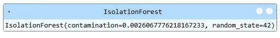
Now we will define the Isolation Forest model. We calculate the fraction of outliers by looking at the number of fraudulent transactions in the dataset then we create and fit the Isolation Forest model with this outlier fraction.
n_estimators=100: Number of trees in the ensemble (improves accuracy).
contamination: Fraction of outliers in data, helps model set detection threshold..
Next we will evaluate the model’s performance by calculating its accuracy in detecting anomalies (fraudulent transactions) based on the anomaly scores.
Decision Function: Computes anomaly scores for each point.
Prediction Adjustment: Converts predictions (1 = normal, -1 = anomaly) to match dataset labels.
Accuracy Calculation: Measures detection rate of anomalies.
Output:
Accuracy in finding anomaly: 0.997175
So we have achieved an accuracy of 99.72% in detecting anomalies with the Isolation Forest model.
Step 5: Comparative Visualization
Now to understand how well the model separates normal and anomalous instances, we will plot the 'Amount' feature to visualize the distinction between normal and fraudulent transactions. We can easily replace 'Amount' with any other feature to visualize its results.
